Exploring radically new modes of musical interaction in live performance
Category: Documentation
Documentation and the speed of an artistic workflow
October 11, 2018
-
During our preparations for the concert at Dokkhuset in May 2018, we had several sessions of combined rehearsal and studio recording. We aimed for doing a recording of the concert and using that for a public release, but wanted to ...
Various presentations and papers 2018
October 11, 2018
-
The crossadaptive project was presented at several conferences in 2018, and several written publications were made. At the NIME conference (New Instruments for Musical Expression) at Virginia Tech, we presented a paper: "Working Methods and Instrument Design for Cross-Adaptive Sessions" ...
Master thesis at UCSD (Jordan Morton)
October 11, 2018
-
Jordan Morton write about the experiences within the crossadaptive project in her master thesis at the University of California San Diego. The title of the thesis is "Composing A Creative Practice: Collaborative Methodologies and Sonic Self-Inquiry In The Expansion Of ...
Concert at Dokkhuset, May 2018
October 11, 2018
-
The project held a concert at Dokkhuset on May 26th. This concert was made as a presentation of the artistic outcome, towards the end of the project. Assuming there is no "final result" of an artistic process, but still representing ...
Crossadaptive seminar Trondheim, November 2017
November 5, 2017
-
As part of the ongoing research on crossadaptive processing and performance, we had a very productive seminar in Trondheim 2. and 3. November (2017). The current post will show the program of presentations, performances and discussions and provide links to ...
Concert and workshop in Oslo
October 30, 2017
-
During "Musikkteknologidagene" (Music Technology Days) at the Norwegian Academy of Music, October 2017, we held a workshop on crossadaptive techniques and also played a set in the evening concert. Here's a video of the concert (thanks for taping it, Daniel ...
Adaptive Parameters in Mixed Music
October 23, 2017
-
Adaptive Parameters in Mixed Music Introduction During the last several years, the interplay between processed and acoustic sounds has been the focus of research at the department of music technology at NTNU. So far, the project “Cross-adaptive processing as musical ...
Session with 4 singers, Trondheim, August 2017
October 9, 2017
-
Location: NTNU, Studio Olavshallen. Date: August 28 2017 Participants: Sissel Vera Pettersen, vocals Ingrid Lode, vocals Heidi Skjerve, vocals Tone Åse, vocals Øyvind Brandtsegg, processing Andreas Bergsland, observer and video documentation Thomas Henriksen, sound engineer Rune Hoemsnes, sound engineer We ...
Session in UCSD Studio A
September 8, 2017
-
This session was done May 11th in Studio A at UCSD. I wanted to record some of the performer constellations I had worked with in San Diego during Fall 2016 / Spring 2017. Even though I had worked with all ...
Playing or being played – the devil is in the delays
June 9, 2017
-
Since the crossadaptive project involves designing relationsips between performative actions and sonic responses, it is also about instrument design in a wide definition of the term. Some of these relationships can be seen as direct extensions to traditional instrument features, ...
The entrails of Open Sound Control, part one
April 7, 2017
-
Many of us are very used to employing the Open Sound Control (OSC) protocol to communicate with synthesisers and other music software. It's very handy and flexible for a number of applications. In the cross adaptive project, OSC provides the ...
Docmarker tool
February 16, 2017
-
Docmarker During our studio sessions and other practical research work sessions, we noted that we needed a tool to annotate documentation streams. The stream could be an audio file, a video or some line of timed events. Audio editors and ...
Crossadaptive session NTNU 12. December 2016
December 16, 2016
-
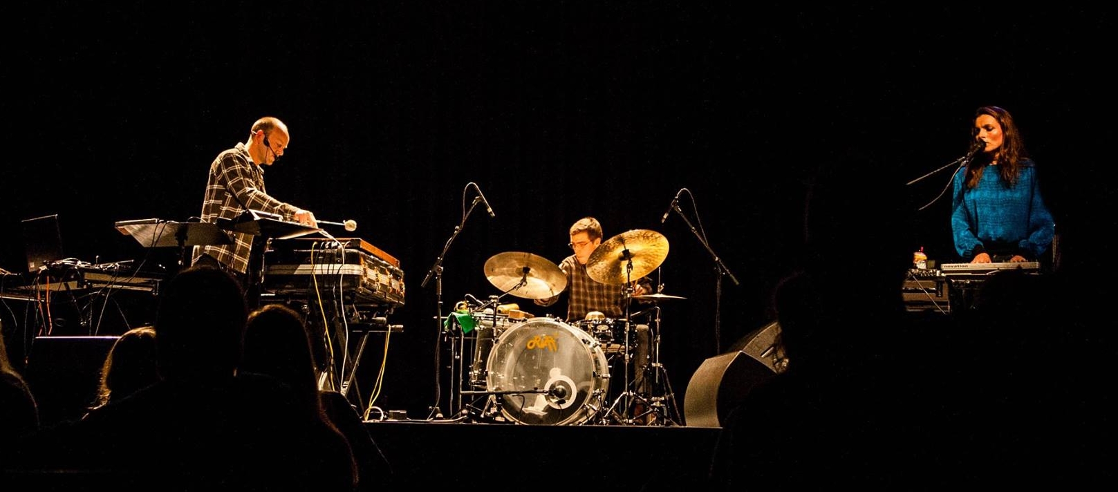
Participants: Trond Engum (processing musician) Tone Åse (vocals) Carl Haakon Waadeland (drums and percussion) Andreas Bergsland (video) Thomas Henriksen (sound technician) Video digest from session: https://www.youtube.com/watch?v=ktprXKVdqF4&feature=youtu.be Session objective and focus: The main focus in this session was to explore other ...
Concerts and presentations, fall 2016
December 15, 2016
-
A number of concerts, presentations and workshops were given during October and November 2016. We could call it the 2016 Crossadaptive Transatlantic tour, but we won’t. This post gives a brief overview. Concerts in Trondheim and Göteborg BRAK/RUG was scheduled ...
Multi-camera recording and broadcasting
November 21, 2016
-
Audio and video documentaion is often an important component of projects that analyse or evaluate musical performance and/or interaction. This is also the case in the Cross Adaptive project where every session was to be recorded in video and multi-track ...
Many of us are very used to employing the Open Sound Control (OSC) protocol to communicate with synthesisers and other music software. It’s very handy and flexible for a number of applications. In the cross adaptive project, OSC provides the backbone of communications between the various bits of programs and plugins we have been devising.
Generally speaking, we do not need to pay much attention to the implementation details of OSC, even as developers. User-level tasks only require us to decide the names of messages addresses, its types and the source of data we want to send. At Programming level, it’s not very different: we just employ an OSC implementation from a library (e.g. liblo, PyOSC) to send and receive messages.
It is only when these libraries are not doing the job as well as we’d like that we have to get our hands dirty. That’s what happened in the past weeks at the project. Oeyvind has diagnosed some significant delays and higher than usual cost in OSC message dispatch. This, when we looked, seemed to stem from the underlying implementation we have been using in Csound (liblo, in this case). We tried to get around this by implementing an asynchronous operation, which seemed to improve the latencies but did nothing to help with computational load. So we had to change tack.
OSC messages are transport-agnostic, but in most cases use the User Datagram Protocol transport layer to package and send messages from one machine (or program) to another. So, it appeared to me that we could just simply write our own sender implementation using UDP directly. I got down to programming an OSCsend opcode that would be a drop-in replacement for the original liblo-based one.
OSC messages are quite straightforward in their structure, based on 4-
byte
blocks of data. They start with an address, which is a null-terminated string like, for instance, “/
foo
/
bar
” :
'/' 'f' 'o' 'o' '/' 'b' 'a' 'r' '\0'
This, we can count, has 9 characters – 9 bytes – and, because of the 4-byte structure, needs to be padded to the next multiple of 4, 12, by inserting some more null characters (zeros). If we don’t do that, an OSC receiver would probably
barf
at it.
Next, we have the data types, e.g. ‘i’, ‘f’, ‘s’ or ‘b’ (the basic types). The first two are numeric, 4-byte integers and floats, respectively. These are to be encoded as big-endian numbers, so we will need to
byteswap
in little-endian platforms before the data is written to the message. The data types are encoded as a string with a starting comma (‘,’) character, and need to conform to 4-byte blocks again. For instance, a message containing a single float would have the following type string:
',' 'f' '\0'
or “,f”. This will need another null character to make it a 4-byte block. Following this, the message takes in a big-endian 4-byte floating-point number. Similar ideas apply to the other numeric type carrying integers.
String types (‘s’) denote a null-terminated string, which as before, needs to conform to a length that is a multiple of 4-bytes. The final type, a blob (‘b’), carries a nondescript sequence of bytes that needs to be decoded at the receiving end into something meaningful. It can be used to hold data arrays of variable lengths, for instance. The structure of the message for this type requires a length (number of bytes in the blob) followed by the byte sequence. The total size needs to be a multiple of 4 bytes, as before. In Csound, blobs are used to carry arrays, audio signals and function table data.
If we follow this recipe, it is pretty straightforward to assemble a message, which will be sent as a UDP packet. Our example above would look like this:
This is what OSCsend does, as well as its new implementation. With it, we managed to provide a lightweight (low computation cost) and fast OSC message sender. In the followup to this post, we will look at the other end, how to receive arbitrary OSC messages from UDP.
During our studio sessions and other practical research work sessions, we noted that we needed a tool to annotate documentation streams. The stream could be an audio file, a video or some line of timed events. Audio editors and DAWs have tools for dropping markers into a file, and there are also tools for annotating video. However, we wanted an easy way of recording timed comments from many users, allowing these to be tied to any sequence of events, wheter recorded as audio, video or in other form. We also wanted each user to be able to make comments without necessarily having access to the file “original”, and for several users to be able to make comments simultaneously. By allowing comments from several users to be merged, one can also use this to do several “passes” of making comments, merging with one’s own previous comments.
Assumedly, one can use this for other kinds of timed comments too. Taking notes on one’s own audio mixes, making edit lists from long interviews, … even marking of student compositions…
The tool is a simple Python script, and the code can be found at
https://github.com/Oeyvind/docmarker
Download, unzip, and run from the terminal with:
python doc_marker.py
The main focus in this session was to explore other analysing methods than used in earlier sessions (focus on rhythmic consonance for the drums, and spectral crest on the vocals). These analysing methods were chosen to get a wider understanding of their technical functionality, but also their possible use in musical interplay. In addition to this there was an intention to include the sample/hold function for the MIDIator plug-in. The session was also set up with a large screen in the live room to monitor the processing instrument to all participants at all times. The idea was to democratize the processing musician role during the session to open up for discussion and tuning of the system as a collective process based on a mutual understanding. This would hopefully communicate a better understanding of the functionality in the system, and how the musicians individually can navigate within it through their musical input. At the same time this also opens up for a closer dialog around choice of effects and parameter mapping during the process.
Earlier experiences and process
Following up on experiences documented through earlier sessions and previous blog posts, the session was prepared to avoid the most obvious shortcomings. First of all, separation between instruments to avoid bleeding through microphones was arranged by placing vocals and drums in separate rooms. Bleeding between microphones was earlier affecting both the analysed signals and effects. The system was prepared to be as flexible as possible beforehand containing several effects to map to, flexibility in this context meaning the possibility to do fast changes and tuning the system depending on the thoughts from the musicians. Since the group of musicians remained unchanged during the session this flexibility was also seen as a necessity to go into details and more subtle changes both in the MIDIator and the effects in play to reach common aesthetical intentions.
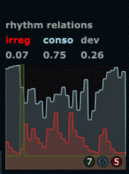
Due to technical problems in the studio (not connected with the cross adaptive set up or software) the session was delayed for several hours resulting in shorter time than originally planned. We therefore made a choice to concentrate only on rhythmic consonance (referred to as rhythmical regularity in the video) as analysing method for both drums and vocals. The method we used to familiarize with this analysing tool was that we started with drums trying out different playing techniques with both regular and irregular strokes while monitoring the visual feedback from the analyser plug-in without any effect. Regular strokes in this case resulting in high stable value, irregular strokes resulting in low value.
Figure 1. Consonance (regularity) visualized in the upper graph.
What became evident was that when the input stopped, the analyser stayed at the last measured value, and in that way could act as a sort of sample/hold function on the last value and in that sense stabilise a setting in an effect until an input was introduced again. Another aspect was that the analysing method worked well for regularity in rhythm, but had more unpredictable behaviour when introducing irregularity.
After learning the analyser behaviour this was further mapped to a delay plugging as an adaptive effect on the drums. The parameter controlled the time range of 14 delays resulting in larger delay time range the more regularity, and vice versa.
After fine-tuning the delay range we agreed that the connection between the analyser, MIDIator and choice of effect worked musically in the same direction. (This was changed later in the session when trying out cross-adaptive processing).
The same procedure was followed when trying vocals, but then concentrating the visual monitoring mostly on the last stage of the chain, the delay effect. This was experienced as more intuitive when all settings were mapped since the musician then could interact visually with the input during performance.
Cross-adaptive processing.
When starting the cross-adaptive recording everyone had followed the process, and tried out the chosen analysing method on own instruments. Even though the focus was mainly on the technical aspects the process had already given the musicians the possibility to rehearse and get familiar with the system.
The system we ended up with was set up in the following way:
Both drums and vocals was analysed by rhythmical consonance (regularity). The drums controlled the send volume to a convolution reverb and a pitch shifter on the vocals. The more regular drums the less of the effects, the less regular drums the more of the effects.
The vocals controlled the time range in the echo plugin on the drums. The more regular pulses from the vocal the less echo time range on the drums, the less regular pulses from the vocals the larger echo time range on the drums.
Sound example (improvisation with cross adaptive setup):
A number of concerts, presentations and workshops were given during October and November 2016. We could call it the 2016 Crossadaptive Transatlantic tour, but we won’t. This post gives a brief overview.
Concerts in Trondheim and Göteborg
BRAK/RUG was scheduled for a concert (with a preceding lecture/presentation) at Rockheim, Trondheim on 21. October. Unfortunately, our drummer Siv became ill and could not play. At 5 in the afternoon (concert start at 7) we called Ola Djupvik to ask if he could sit in with us. Ola has experience from playing in a musical setting with live processing and crossadaptive processing, for example the Session 20. – 21 September, and also from performing with music technology students Ada Mathea Hoel, Øystein Marker and others. We were very happy and grateful for his courage to step in on such short notice. Here’s and excerpt from the presentation that night, showing vocal pitch controlling reverb on the drums (high pitch means smaller reverb size), transient density on the drums controlling delay feedback on the vocals (faster playing means less feedback).
There is a significant amount of crossbleed between vocals and drums, so the crossadaptivity is quite flaky. We still have some work to do on source separation to make this work well when playing live with a PA system.
Thanks to Tor Breivik for recording the Rockheim event. The clip here shows only the crossadaptive demonstration. The full concert is available on
Soundcloud
Brandtsegg, Ratkje, Djupvik trio at Rockheim
The day after the Trondheim concert, we played at the Göteborg Art Sounds festival. Now, Siv was feeling better and was able to play. Very nice venue at Stora Teatern. This show was not recorded.
And then we take… the US
The crossadaptive project was presented at the
Transatalantic Forum
in Chicago on October 24, in a special session titled “
Sensational Design: Space, Media, and the Senses
”. Both Sigurd Saue, Trond Engum and myself (Øyvind Brandtsegg) took part in the presentation, showing the many-faceted aspects of our work. Being a team of three people also helped the networking effort that is naturally a part of such a forum. During our stay in Chicago, we also visited the School of the Art Institute of Chicago, meeting Nicolas Collins, Shawn Decker, Lou Mallozzi, and Bob Snyder to start working on exchange programs for both students and faculty. Later in the week, Brandtsegg did a presentation of the crossadaptive project during a SAIC class on audio projects.
Sigurd Saue and Bob Snyder at SAIC
After Chicago, Engum and Saue went to Trondheim, while I traveled further on to San Francisco, Los Angeles, Santa Barabara, and then finally to San Diego.
In the Bay area, after jamming with Joel Davel in Paul Dresher’s studio, and playing a concert with Matt Ingalls and Ken Ueno at Tom’s Place, I presented the crossadaptive project at CCRMA, Stanford University on November 2. The presentations seemed well received and spurred a long discussion where we touched on the use of MFCC’s, ratios and critical bands, stabilizing of the peaks of rhythmic autocorrelation, the difference of the correlation between two inputs (to get to the details of each signal), and more. Getting the opportunity to discuss audio analysis with this crowd was a treat. I also got the opportunity to go back the day after to look at student projects, which I find gives a nice feel of the vibe of the institution. There is a video of the presentation here
After Stanford, I also did a presentation at the beautiful CNMAT at UC Berkeley, with Ed Campion, Rama Gottfried, a group of enthusiastic students. There I also met colleague P.A. Nilsson from Göteborg, as he was on a residency there. P.A.’s current focus on technology to intervene and structure improvisations is closely related to some of the implications of our project.
CNMAT, UC Berkeley
On November 7 and 8, I did workshops at California Institute of the Arts, invited by Amy Knoles. In addition to presenting the technologies involved, we did practical studies where the students played in processed settings and experienced the musical potential and also the different considerations involved in this kind of performance.
Calarts workshops
Clint Dodson and Øyvind Brandtsegg experimenting together at CalArts
At UC Santa Barbara, I did a presentation in Studio Xenakis on November 9. There, I met with Curtis Roads, Andres Cabrera, and a broad range of their colleagues and students. With regards to the listening to crossadaptive performances, Curtis Roads made a precise observation that
it is relatively easy to follow if one knows the mappings, but it could be hard to decode the mapping just by listening to the results
. In Santa Barbara I also got to meet Owen Campbell, who did a master thesis on crossadaptive and got insight into his research and software solutions. His work on
ADEPT
was also presented at the AES workshop on intelligent music production at Queen Mary University this September, where Owen also met our student Iver Jordal, presenting his research on
artificial intelligence in crossadaptive processing.
San Diego
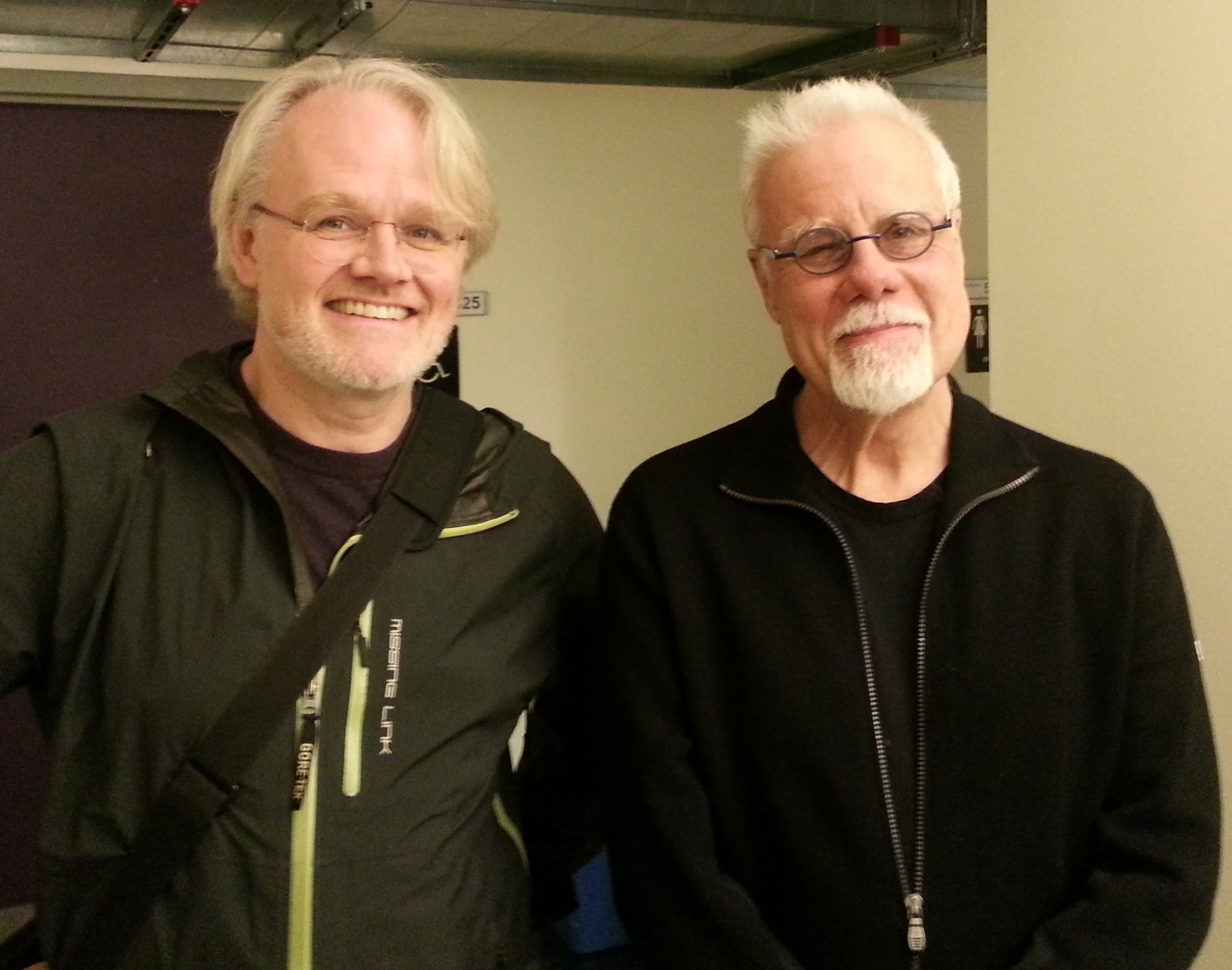
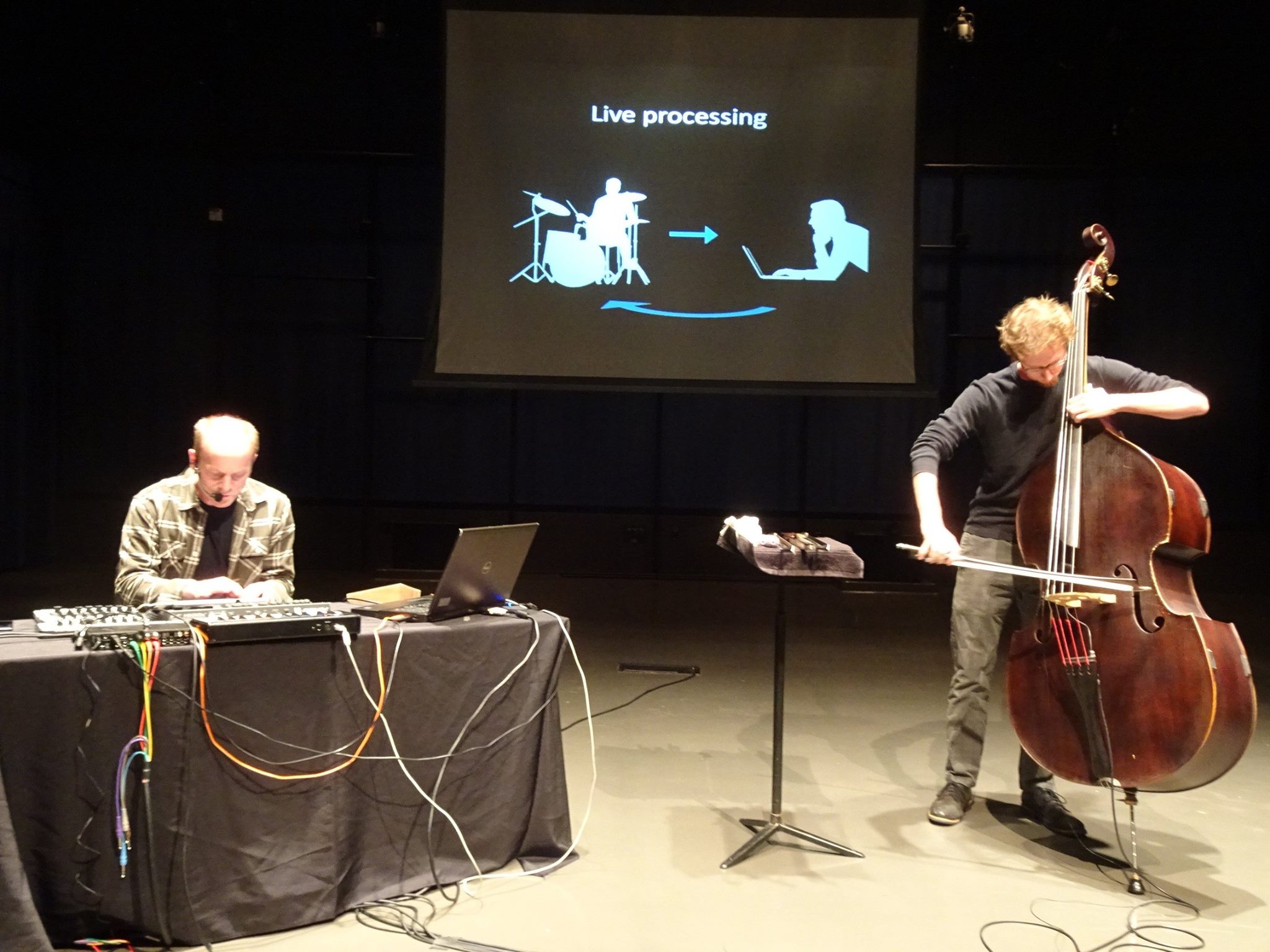
Back in San Diego, I did a combined presentation and concert for the computer music forum on November 17. I had the pleasure of playing together with Kyle Motl on double bass for this performance.
Kyle Motl and Øyvind Brandtsegg, UC San Diego
We demonstrated both live processing and crossadaptive processing between voice and bass. There was a rich discussion with the audience. We touched on issues of learning (one by one parameter, or learning a combined and complex parameter set like one would do on an acoustic instrument), etudes, inverted mapping sometimes being more musically intuitive, how this can make a musician pay more attention to each other than to self (frustrating or liberating?), and tuning of the range and shape of parameter mappings (still seems to be a bit on/off sometimes, with relatively low resolution in the middle range).
First we did an example of a simple mapping:
Vocal amplitude reduce reverb size for bass,
Bass amplitude reduce delay feedback on vocals
Then a more complex example:
Vocal
transient
density
-> Bass
filter
frequency
of a lowpass filter
Vocal
pitch
-> Bass
delay
filter frequency
Vocal
percussive
-> Bass
delay
feedback
Bass
transient
density
-> Vocal
reverb
size
(less)
Bass
pitch+centroid
-> Vocal
tremolo speed
Bass
noisiness
-> Vocal
tremolo
grain
size
(less)
We also demonstrated another and more direct kind of crossadaptive processing, when doing convolution with live sampled impulse response. Oeyvind manually controlled the IR live sampling of sections from Kylse’s playing, and also triggered the convolver with tapping and scratching on a small wooden box with a piezo microphone. The wooden box source is not heard directly in the recording, but the resulting convolution is. No other processing is done, just the convolution process.
We also played a longer track of regular live processing this evening. This track is available on
Soundcloud
Thanks to UCSD and recording engineers Kevin Dibella and James Forest Reid for recording the Nov 17 event.
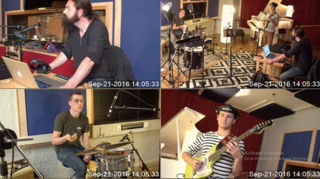
Audio and video documentaion is often an important component of projects that analyse or evaluate musical performance and/or interaction. This is also the case in the Cross Adaptive project where every session was to be recorded in video and multi-track audio, and subsequently within two days, this material should be organized and edited into a 2-5 minute digest. However, when documenting sessions in this project we face the challenge of having several musicians located in one room (the studio recording room), often so that they are facing each other rather than being oriented in the same direction. Thus, an ordinary single camera recording of the musicians would have difficulties including all musicians in one image. Our challenge, then, has been to find some way of doing this that has high enough quality to be able to detect salient aspects of the musical performances, that is in sync both for video streams and audio, and but isn’t too expensive, since the budget for this work has been limited, or too complicated to handle. In this blog post I will present some of the options I have considered, both in terms of hardware and software, and present some of the tests I have done in the process.
Commercial hardware/software solutions
One of the things we considered in the first investigative phase was to check the commercial market for multi-camera recording solutions. After some initial searches on the web I made a few inquiries, which resulted in two quotes for two different systems:
Both included all hardware and software needed for in-sync multi-camera recording, except for the cameras in themselves. The StreamPix quote also included a computer with suitable specs. Both quotes were immediately deemed inadequate since prices were well beyond our budget (> $5000).
I also have to mention that after having set up a system for the first session in September 2016, we have seen the Apollo multicamera recorder/switcher, which looks like a very light weight and convenient way of doing multi-camera recording:
At $2.995 (price listed on the US web site), it might be a possibility to consider in the future, even if it still is in the high end of our budget range.
Using PCs and USB3 cameras
A project currently running at the NTNU (in collaboration with NRK and UNINETT) is Nettmusikk (Net Music). This project is testing solutions to do high-resolution, low latency streaming of audio and video over the internet. The project has bought four USB3 cameras (Point Grey Grasshopper, GS3-U3-41C6C-C) and four dual boot (Linux/win) PCs with high-performance specs. These cameras deliver a very high quality image with low latency. However, one challenge is that the USB3 standard is still not very developed so that cameras can “plug-and-play” on all platforms, and specifically that the software and drivers for the Point Grey cameras is proprietary, and won’t therefore provide images for all software out-of-the-box.
After doing some research on the Point Grey camera solution, we found that there were several issues that made this option unsuitable and/or impractical.
1. To get full sync between cameras, they needed to have an optical strobe sync, which required a master/slave configuration with all cameras to in the same room.
2. There was no software that could do multi-camera recording from USB3 out-of-the-box. Rather, Point Grey provided an SDK (Fly Capture) with working examples that allowed building of our own applications. While this was an option we considered, it still looked like an option that demanded a bit of programming work (C++).
3. Because the cameras stream and record in raw we would also need very fast SSDs to record 4 video files at once. If we were recording 4 video streams at 8-bit 1920×1080 @ 30 FPS that would be 248.8 mb/s (62.2 x 4) of data. This would also fill up hard drive space pretty fast.
USB2 HD cameras
It turned out that one of the collaborators in the Nettmusikk project had access to four USB2 HD cameras. Since the USB2 protocol is a cross-platform standard that provides plug-and-play and usually has few issues with compatibility. The quality of these Tanberg Precision HD cameras was far from professional production quality, but had reasonably clear images. When viewing the camera image on a computer, there was a barely noticable latency. Here is a review made by the gadgeteer:
Without high-quality lenses, however, the possibilities for adjusting zoom, angle and light sensiticity were non-existent, and particularly the latter proved to be an issue in the sessions. Especially we went into problems if direct light sources were in the image, so that careful placement of light sources was necessary. Also, it was sometimes difficult to get enough distance between the cameras and the performer since the room wasn’t very big, and an adjustable lens would probably have been of help here. Furthermore, the cameras has an autofocus function that sometimes was confused in the first session, making the image blurry for a second or two, until it was appropriately adjusted. Lastly, the cameras had a foot suitable for table placement, but no possibilities of fastening it to a standard stand, like the Point Grey camera has. I therefore had to use duck tape to fasten the cameras, which worked ok, but looked far from professional.
A second issue for concern was whether these cameras could provide images with long cable lengths. What I learned here was that they would operate perfectly with an 5m USB extension if they were connected to a powered hub at the end, that provided the cameras with sufficient power. It turned out that two cameras per hub did work, but might sometimes introduce some latency and drop-outs. Thus, taking the signal from four cameras via four hubs and extension chords into the four USB ports on the PC seemed like the best solution. (Although we only used three hubs in the first session). That gave us a fairly high flexibility in terms of placing the cameras.
Mosaic image
Due to the very high amounts of data involved in dealing with multiple cameras, using instead a composite/ mosaic gathering all four images into one, seemed like a possible solution. Arguably, it would going from HD to HD/4 per image. Still, this option had the great advantage of making post-production switching between cameras superfluous. And since the goal in this project was to produce a 2-5 minute digest in two days this seemed like a very attracive option. The question was then how to collate and sync four images into one without any glitches or hiccups. In the following, I will present the four solutions that was tested:
1. ffmpeg (
https://www.ffmpeg.org/
)
ffmpeg is an open source command line software that can do a number of different operation on audio and video streams and files; recording, converting, filtering, ressampling, muxing, demuxing, etc. It is highly flexible and customizable with the cost of having a steep user threshold with cumbersome operation, since everything has to be run at command line. The flexibility and the fact that it was free still made it an option to consider.
ffmpeg could be easily installed OSX from pre built binaries. On Windows it also has to be built from sources with the mingw-w64 project (see
https://trac.ffmpeg.org/wiki/CompilationGuide/MinGW
). This option seemed like a bit of work, but at the time when it was considered, it still sounded like a viable option.
After some initial tests based on examples in the ffmpeg wiki (
https://trac.ffmpeg.org/wiki
) I was able to run the following script as a test on OSX:
The script produced four streams of video, one from the an external web camera and three from the internal Face Time HD camera. However, the individual images were far from in sync, and seemed to loose the stream and/or lag behind several seconds at a time. This initial test plus the sync issues and the prospects of a time consuming build process on Windows made me abandon the ffmpeg solution.
2. Processing
Using Processing, described as a “flexible software sketchbook and a language for learning how to code within the context of the visual arts” (
https://processing.org/
), seemed like a more promising path. Again I relied on examples I located on the web and put together a sketch that seemed to do what we were after (I also had to install the video library to be able to run the sketch).
void setup(){
size(1280, 720);
cameras=Capture.list();
println(“Available cameras:”);
for (int i = 0; i < cameras.length; i++) {
println(cameras[i], i);
}
/// Choose cameras with the appropriate number from the list and corresponding resolution
/// Here I had to look in the printout list to find the correct numbers to enter
camA = new Capture(this,640,360,cameras[18]);
camB = new Capture(this,640,360,cameras[3]);
camC = new Capture(this,640,360,cameras[33]);
camA.start();
camB.start();
camC.start();
}
void draw() {
image(camA, 0, 0, 640,360);
image(camB, 640, 0, 640,360);
image(camC, 0, 360, 640,360);
}
This sketch nicely gathered the images from three cameras into my mac, with little latency (approx. 50-100 ms). This made me opt to go further and port the sketch to Windows. After installing Processing on the win-PC and running the sktetch there however, I could only get one image out at a time. My hypothesis was that the problem came from all the different cameras having the same number in the list of drivers. These problem made me abandon Processing in search for simpler solutions.
3. IP Camera Viewer
After doing some more searches, I came across IP Camera viewer (
http://www.deskshare.com/ip-camera-viewer.aspx
), a free and light-weight application for different win versions, with support for over 2000 cameras according to their web site. After some initial tests, I found that this application was a quick and easy solution to what we wanted in the project. I could easily gather up to four camera streams in the viewer and the quality seemed good enough to capture details of the performers. It was also very easy to set up and use, and also seemed stable and robust. Thus, this solution turned out to be what we used in our first session, and it gave us results that were good enough in quality for performance analysis.
4. VLC (
http://www.videolan.org/vlc/
)
The leader of the Nettmusikk project, Otto Wittner, made a VLC script to produce a mosaic image, albeit with only two images:
# Webcam no 1
new ch1 broadcast enabled
setup ch1 input v4l2:///dev/video0:chroma=MJPG:width=320:height=240:fps=30
setup ch1 output #mosaic-bridge{id=1}
# Webcam no 2
new ch2 broadcast enabled
setup ch2 input v4l2:///dev/video1:chroma=MJPG:width=320:height=240:fps=30
setup ch2 output #mosaic-bridge{id=2}
# Background surface (image)
new bg broadcast enabled
setup bg input bg.png
# Add mosaic on top of image, encode everything, display the result as well as stream udp
setup bg output #transcode{sfilter=mosaic{width=640,height=480,cols=2,rows=1,position=1,order=”1,2″,keep-picture=enabled,align=1},vcodec=mp4v,vb=5000,fps=30}:duplicate{dst=display,dst=udp{dst=streamer.uninett.no:9400}}
setup bg option image-duration=-1 # Make background image be streamed forever
#Start everything
control bg play
control ch1 play
control ch2 play
While it seemed to work well on Linux with two images, the fact that we already had a solution in place made it natural not to persue this solution further at the time.
5. Other software
Among other software I located that could gather several images into one was CaptureSync (
http://bensoftware.com/capturesync/
). This software was for mac only, and was therefore not tested.
Screen capture and broadcast
Another important function that still wasn’t covered with the IP camera viewer was recording. Another search uncovered many options here, most of them directed towards gaming capture. The first of these I tested was OBS, Open Broadcaster Software (
https://obsproject.com/
). This open source software turned out to do exactly what we wanted and more, so this became the solution we used at the first session. The software was easily setup to record from the desktop with a 30fps frame rate and close to HD quality with output set to .mp4. There was, however, a noticable lag between audio and video, with video lagging behind approximately 50-100ms. This was corrected in post-production editing, but could potentially have been solved with inserting a delay on the audio stream until it was in sync. Also there were occasional clicks in the audio stream, but I did not have time to figure out whether this was caused by the software or the (internal) sound device we used for recording. We will do more tests on this matter later. The recordings were started with a clap to allow for post-sync.
Surprisingly, OBS was very easy to set it up for live-streaming. I used my own YouTube account where I set up for the Stream Now option (
https://support.google.com/youtube/answer/2853700?hl=en
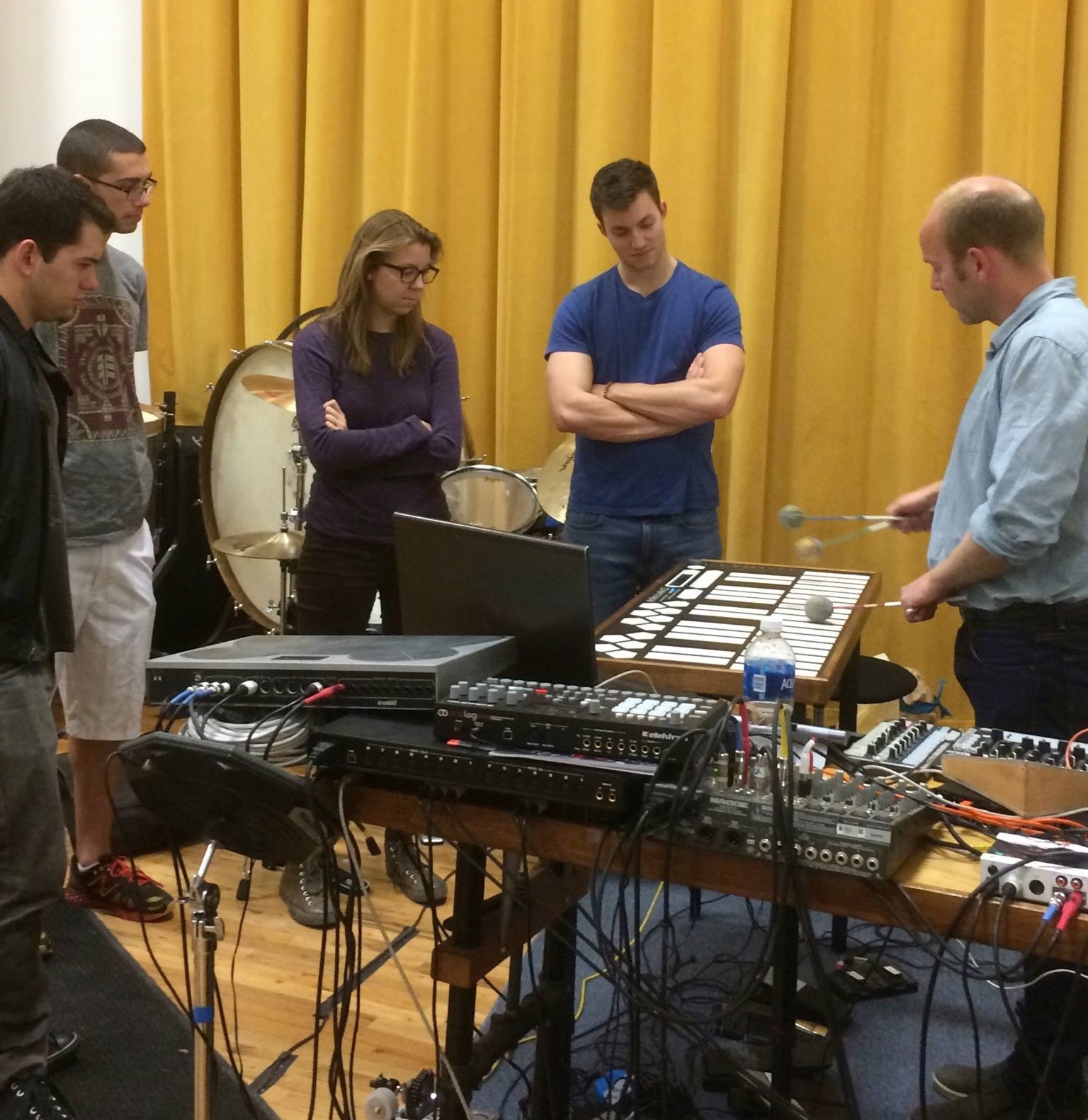
). This gave me a a key code that I could copy into OBS, and then simply press the “Start streaming” button. The stream had a lag of about 10 seconds, but had a good quality and consistence. Thereby we had easily set up something we only considered as optional to begin with. Øyvind was very pleased to be able to follow the last part of the first session from his breakfast table in San Diego!
Live stream from session with jazz students
Custom video markup solution
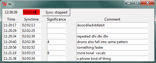
Øyvind wrote a small command line program in python that could generate a time-code based list of markers to go with the video. When pressing a number one could indicate when (number of seconds before pressing) a comment was to be inserted relative to a custom set timer. This made it possible to easily synchronize with the clock that IP Camera Viewer printed on top of the video images. Moreover, it allowed rating significance. Although it required a little bit of practice, I found it useful for making notes during the session, as well as when going through the post-session interview videos. One possible way of improving it would be to have a program that could merge and order (in time) comments made either in different run throughs or by different commentators.
Editing
After two days of recording the videos were to be edited down to a single five minute video. After some testing with free software like iMovie (mac) and MovieMaker (win), I abandoned both options due to lack of options and intuitive use. After a little bit of serching I discovered Filmora from Wondershare (
http://filmora.wondershare.com/
), which I tried out as a free demo before I decided to buy it ($29.90 for a 1-year license). In my view, it was lightweight, had sufficient options to do simple editing and it was quick and easy to use.
Conclusions
We ended up with a multicamera recording and live-streaming solution that was easy to use and very cheap to set up. The only expenses we have had so far has been USB extension cords and hubs as well as the Filmora editor, which was also cheap. Although we do not have our own cameras yet, the prices of new USB2 cameras would not imply a big cut into the budget, if we need to buy four of them. Moreover, finding free software that gave us what we wanted out-of-the-box was a huge relief after intital tests with software like ffmpeg, Processing and VLC.