As I have discussed before in my previous post, as part of this project we have been selecting a number of useful operations to implement in Csound, as part of its array opcode collection. We have looked at the components necessary for the implementation of the Mel-frequency cepstrum coefficient (MFCC) analysis and in this post I will discuss the Mel-frequency filterbank as the final missing piece.
The word filterbank might be a little misleading in this context, as we will not necessarily implement a complete filter. We will design a set of weighting curves that will be applied to the power spectrum. From each one of this we will obtain an average value, which will be the output of the MFB at a given centre frequency. So from this perspective, the complete filter is actually made up of the power spectrum analysis and the MFB proper.
So what we need to do is the following:
- Find L evenly-space centre frequencies in the Mel scale (within a minimum and maximum range).
- Construct L overlapping triangle-shape curves, centred at each Mel-scale frequency.
- Apply each one of these curves to the power spectrum and averaging the result. These will be the outputs of the filterbank.
The power spectrum input comes as sequence of equally-spaced bins. So, to achieve the first step, we need to convert to/from the Mel scale, and also to be able to establish which bins will be equivalent to the centre frequencies of each triangular curve. We will show how this is done using the Python language as an example.
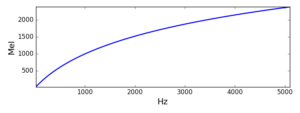
The following function converts from a frequency in Hz to a Mel-scale frequency.
import pylab as pl
def f2mel(f):
  return 1125.*pl.log(1.+f/700.)

With this function, we can convert our start and end Mel values and linearly space the L filter centre frequencies. From these L Mel values, we can get the power spectrum bins using
def mel2bin(m,N,sr):
  f = 700.*(pl.exp(m/1125.) - 1.)
  return  int(f/(sr/(2*N)))
where m is the Mel frequency, N is the DFT size used and sr is the sampling rate. A list of bin numbers can be created, associating each L Mel centre frequency with a bin number
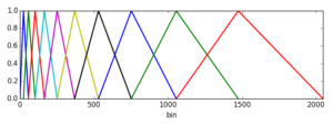
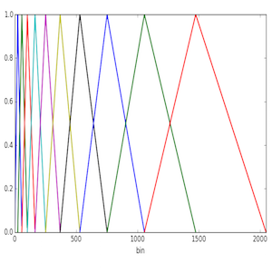
Step 2 is effectively based on creating ramps that will connect each bin in the list above. The following figure demonstrates the idea for L=10, and N=4096 (2048 bins)

Each triangle starts at a Mel frequency in the list, rises to the next, and decays to the following one (frequencies are quantised to bin centres). To obtain the output for each filter we weigh the bin values (spectral powers) by these curves and then output the average value for each band.
The Python code for the MFB operation is shown below:
def MFB(input,L,min,max,sr):
  """
  From a power spectrum in input, creates an array
  consisting of L values containing
  its MFB, from a min to a max frequency sampled
  at sr Hz.
  """
  N = len(input)
  start = f2mel(min)
  end = f2mel(max)
  incr = (end-start)/(L+1)
  bins = pl.zeros(L+2)
  for i in range(0,L+2):
    bins[i] = mel2bin(start,N-1,sr)
    start += incr
  output = pl.zeros(L)
  i = 0
  for i in range(0,L):
    sum = 0.0
    start = bins[i]
    mid = bins[i+1]
    end = bins[i+2]
    incr =  1.0/(mid - start)
    decr =  1.0/(end - mid)
    g = 0.0
    for bin in input[start:mid]:
      sum += bin*g
      g += incr
    g = 1.0
    for bin in input[mid:end]:
      sum += bin*g
      g -= decr
    output[i] = sum/(end - start)
  return output
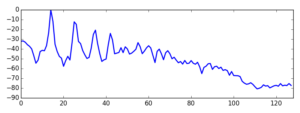
We can demonstrate the use of the MFB by plotting the output of a N=4096, L=128 full-spectrum magnitude analysis of a flute tone.

We can see how the MFB identifies clearly the signal harmonics. Of course, the original application we had in mind (MFCCs) is significantly different from this one, but this example shows what kinds of outputs we should expect from the MFB.

