Documentation and the speed of an artistic workflow

During our preparations for the concert at Dokkhuset in May 2018, we had several sessions of  combined rehearsal and studio recording. We aimed for doing a recording of the concert and using that for a public release, but wanted to record the preparations too, in case we needed additional (or backup) material. We ended up using a combinations of the live and studio recordings for the upcoming release, so in that respect the strategy worked as planned.

Since we already had a substantial documentation of practical experiments from earlier sessions, we decided to not document these sessions with video and written reflections. One could of course say that the sessions are still documented with audio recordings, although I would characterize these different modes of documentation so differently that they require different treatment and impacts the production and the reflection if very different ways. We as musicians are quite used to working in the studio, used to being recorded, and familiar with the scrutiny that follows from this process. Close miking in an optimal recording environment brings out details that you would not necessarily notice otherwise.  The impact of the difference in documentation methods and documentation purpose is the aim of this blog post.

4-camera video documentation

During the practical sessions earlier in this project, we had done what I would call a full video documentation. This consisted of a written session report form (with objectives, listing of participants and takes, reflections during and after the session), a 4-camera video recording of the full session, with reflection interviews after the session, a video digest with highlights of the raw video takes, and a blog post summing up and presenting the results. This recipe was developed as a collaboration between Andreas Bergsland and myself, with Bergsland leading the interviews and taking care of all parts of the video production. A documentation software tool (docmarker) was also developed by me, to aid in marking significant moments in time during sessions, with the purpose of speeding up the process of sifting through the material when editing.

Docmarker tool

Such an extensive documentation format of course requires substantial resources, but care was taken to try to ensure that the artistic process should not be slowed down by documentation work. We had dedicated personell doing the documentation, for most sessions Bergsland would transparently take care of the video production. The reflective interviews were done after all performing activities were completed, and we also had considerable technical assistance from studio engineers (led by Thomas Henriksen). All this should ensure that any burden of documentation should not impose any hindrance to the workflow of the artistic process being documented.

Still, when we did these final rehearsals in May 2018 without this kind of documentation, I realized that the process and the workflow was much faster. It seems for me like the act of being documented influence the flow of the process in a very significant manner. I relate this to a difference between a pure artistic process, and an artistic research process. I do not propose that what I say here has any form of general validity, but I do recognize it within my own experience from this project and from earlier artistic research projects. It appears to be related to being aware of one’s own intentions on an intellectual level, as opposed to “just doing”. During my doctoral research project “New creative possibilities through improvisational use of compositional techniques, – a new computer instrument for the performing musician” finished in 2008, I also noted this difficulty of doing research on my own process. The being inside while looking from the outside.  The intuitive and the analytic. The subjective and the attempt at being objective. During an earlier session in the crossadaptive project, Bergsland asked me right after a take what I had done during that take. I replied that I did exactly what I said I should (before the take). He then noted that it did not sound as if this was what happened, and I needed to check my settings and realized, yes, … I had actually done some adjustments early in the take “just to make it work”.

After this insight in the May sessions, I have discussed this issue with several collagues. Many seem to agree with me that it would be interesting to try to document the moment when an artistic process ignites, the moment when “it happens”. Many also recognize the inevitable slowdown due to an analytical component being introduced into the inner loop of the process. Others would say that I must be doing something wrong if the act of documentation slows me down so much. The way I experience this, the artistic process has several layers, each with it’s own iteration time. Parts of the process iterates on the time scale of years, where reflective insight and slow learning influence the growth of ideas. Other intermediary layers also exist as onion skin layers before we get to the inner loop that is active during performance. Here, the millisecond interactions between impulses and reactions is at the most sensitive to interruptions and distractions. Any kind of small drag at this level impedes the flow and slows down the loop, sometimes to the extent that it will not work, it stops. As if it was a rotating wheel with a self-preserving spin, delicately balancing between friction and flow. On the longer time scales, documentation does not imede the process, but rather it can enrich it. On those time scales I also recognize the accumulation of material, of background research, technical solutions, philosophical perspectives and so on. It may seem like the gunpower to allow something to ignite is collected during those longer loops, while the spark… well that is a fickle and short-lived entity more vulnerable to analytical impact. In quantum physics there are also (as far as I know) particles too small to be observed, where the act of observation collapses a potentiality. Maybe there is a similar uncertainty principle in artistic research?

Master thesis at UCSD (Jordan Morton)

Jordan Morton write about the experiences within the crossadaptive project in her master thesis at the University of California San Diego. The title of the thesis is “Composing A Creative Practice: Collaborative Methodologies and Sonic Self-Inquiry In The Expansion Of Form Through Song”. Jordan was one of the performers that took part in several sessions, experiments and productions. Her master thesis give a valuable report of how the collaboration was experienced by her, and how it contributed to some new directions of inquiry within the practical part of her master.

Full text available here:
https://escholarship.org/uc/item/0641v1r0

Crossadaptive seminar Trondheim, November 2017

As  part of the ongoing research on crossadaptive processing and performance, we had a very productive seminar in Trondheim 2. and 3. November (2017). The current post will show the program of presentations, performances and discussions and provide links to more detailed documentation of each session as it becomes available. Each part will be added as the documentations is ready, so if something is missing now, do check back later. The seminar was also streamed here , and the recorded streams will be archived.

In addition to the researchers presenting, we also had an audience of students from the music technology and the jazz departments, as well as other researchers and teachers from NTNU. We are grateful for the input from the audience to enrich our discussions.

Program:

Thursday 2. November

Practical experiments

Introduction and status. [slides]
Øyvind Brandtsegg

Performance
Maja S.K. Ratkje, Øyvind Brandtsegg, Miller Puckette (standin for Stian Westerhus)

Work methods and session reports. Experiences, insights, reflections.
Trond Engum (with team) [slides] ,  Bernt Isak Wærstad (with team) [slides]

Instruments and tools

Instrumental affordances, crossadaptivity as instrumental gesture.
Marije Baalman [slides]


Performance
Tone Åse, Carl Haakon Waadeland, Trond Engum

Instrument design and technological developments. [slides]
Sigurd Saue, Victor Lazzarini, Øyvind Brandtsegg

Friday 3. November

Reflection. Aesthetic and philosophical issues

Documentation methods [slides]
Andreas Bergsland


Performance
Bjørnar Habbestad, Gyrid N. Kaldestad, Bernt Isak Wærstad

What does it mean for the performer, for the audience, for the music? How does it change the game?
Solveig Bøe [notes] , Simon Emmerson [slides]

Wider use and perspectives

Experiences with Philippe Manoury and Juliana Snapper, thoughts on instrumental control, and a performance
Miller Puckette [PD patches]
(with Øyvind Brandtsegg for a brief liveconvolver performance)

Looking at the music from the mix perspective. Viability of effects as expression. The wider field of automatic mixing and adaptive effects.
Gary Bromham [slides ], Josh Reiss [slides]

Outcomes and evaluation. [slides]
Moderator: Øyvind Brandtsegg

Adaptive Parameters in Mixed Music

Adaptive Parameters in Mixed Music

Introduction

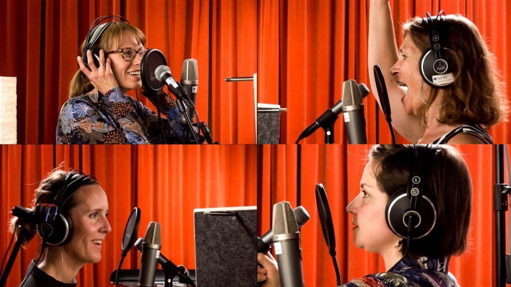
During the last several years, the interplay between processed and acoustic sounds has been the focus of research at the department of music technology at NTNU. So far, the project “Cross-adaptive processing as musical intervention” has been mainly concerned with improvised music such as shown with the music of T-EMP. However, through discussions with Øyvind Brandtsegg and several others at NTNU, I have come to find several aspects of their work interesting in the world of written composition, especially mixed music. Frengel (2010) defines this as a form of electroacoustic music which combines a live and/or acoustic performer with electronics. During the last few years I have especially come to be interested in Philippe Manoury’s conception of mixed music which he calls real-time music ( la musique du temps réel ). This puts emphasis on the idea of real-time versus deferred time which we will come back to later in this article.

The aspect of the cross-adaptive synthesis project which makes the most resonance with mixed music is the idea of adaptive parameters in its most basic form. A parameter X of a sound, influences parameter Y of another sound. To this author, this idea can be directly correlated to Philippe Manoury’s conception of partitions virtuelles which could be translated into English as virtual partition or sheet music. In this article, we will explore some of the links between these concepts, and especially how they can start to influence our compositional practices in mixed music. A few examples of how a few composers have used adaptive parameters will also be given. It is also important to point out that the composers named in this article are far from being the only ones using adaptive parameters, they have done it in either an outstanding and/or very pedagogical way when it comes to the technical aspect of adaptive parameters.

Partitions virtuelles, R elative Values & Absolute Values

Let us first establish the term virtual partition. Manoury’s (1997) conception comes originally from discussions with the late Pierre Boulez, although it was Manoury that expanded on the concept and extended it through Compositions such as “En écho” (1993-1994), “Neptune” (1991), and “Jupiter” (1987).

Virtual partition is a concept that refers directly to the idea of notation as it is used with traditional acoustic music. If we think of Beethoven’s piano sonatas, the notation tells us which notes to play (ie. C4 followed by E4, etc). It might also contain some tempo marks, dynamic markings and phrasing. Do these parameters form the complete list of parameters that a musician can play? The simple answer is no. These are only basic, and often parameters of relative value. A fortissimo symbol does not mean “play at 90 dB”, the symbol is relative compared to what has come before and what will come after. The absolute parameter that we have in this case, is the notes that are written in the sheet music. An A4 will remain an A4. This duality of seeing absolute against relative is also what has given us the world of interpretation. Paul Lewis will not play the same piece in the exact same way as András Schiff even though they will be playing the exact same notes. This is a vital part of the richness of the classical repertoire: its interpretation.

As Manoury points out, in early electroacoustic music this possibility of interpretation was not possible. The so-called “tyranny of tape” made it rather difficult to have more relative values, and in fact also limited the relative values of the live musicians as their tempo and dynamics had to take into consideration a medium that could not be changed then and there. This aspect of the integration of the electronics is a large field into itself which interests this author very much. Although an exhaustive discussion of this is far beyond the scope of this article, it should be noted that adaptive parameters can be used with most of these integration techniques. However, at this point this author does believe that score following and its real-time relative techniques permit this level of interactivity on a higher plane than say the scene system such as in the piece “Lichtbogen” (1986-1987) by Kaija Saariaho where the electronics are set at specific levels until the next scene starts.

Therefore, the main idea of the virtual partition is to bring interpretation into the use of electronics within mixed music. The first aspect to be able to do so is to work with both relative and absolute variables. How does this relate to adaptive parameters? By using electronics that have several relative values that are influenced either by the electronics themselves, the musician(s) or a combination of both, it becomes possible to bring interpretation to the world of electronics. In other words, the use of adaptive parameters within mixed music can bring more interpretation and fluidity into the genre.

Time & Musical Time

The traditional complaint and/or reason for not implementing adaptive parameters/virtual partitions in mixed music has been its difficulty. The Cross-adaptive synthesis project has proven that complex and beautiful results can be made with adaptive parameters. The flexibility of the electronics can only make the rapport between the musicians and computer a more positive one. Another reason that has often been cited is if the relationships would be clear to the listener. This author feels that this criticism is slightly oblique. The use of adaptive parameters may not always be heard by the audience, but it does influence how much the performer(s) feel connected to the electronics. It is also the basis of being able to create an electronic interpretation. Composers like Philippe Manoury for example, believe that the use of a real-time system with adaptive parameters is the only way to preserve the expressivity while working between electronic and acoustic instruments (Ramstrum, 2006).

Another problem that has often come up when it comes to written music, is how to combine the precise activity of contemporary writing with a computer? Back in the 80’s composers like Philippe Manoury often had to use the help of programmers such as Miller Puckette to come up with novel ideas (which in their case would later lead to the development of MaxMSP and Pure Data). However, the arrival of more stable score followers and recognizers (a distinction brought to the light in Manoury, 1997, p.75-78) has made it possible to think of electronics within musical time (ex. quarter note) instead of absolute time (ex. milliseconds). This also allows a composer to further integrate the interpretation of the electronics directly into the language of the score. One could understand this as the computer being able to translate information from a musical language to a binary language.

To give a simple example, we can assume that the electronic process we are controlling is a playback file on a computer. In the score of our imaginary piece, in 5 measures the solo musician must go from fortissimo to pianissimo and eventually fading out niente (meaning gradually fading to silence). As this is happening, the composer would like the pitch of the playback file to rise, as the amplitude of the musician goes down. In absolute time, one would have to program the number of milliseconds each measure should take and hope that the musician and computer would be in sync. However, by using relative time it is easier, as one can tell the computer that the musician will be playing 5 measures. If we combine this with adaptive parameters, we can directly (or indirectly, if preferred) connect the amplitude of the musician to the pitch of the playback for those 5 measures. This idea, which seemed to be most probably a dream for composers in the 80’s has now become reality  because of programs like Antescofo (described in Cont, 2008) as well as the concept of adaptive parameters which is becoming more commonplace.

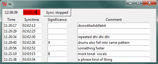
The use of microphones and/or other sensors allows us to extract more information from the musician(s) and one can connect these to specific parameters however directly or indirectly one wishes. Øyvind Brandtsegg’s software also allows the extraction of many features of sound(s) and map these to audio processing parameters. In combination with a score follower or other integration methods, this can be an incredibly powerful tool to organize a composition.

Examples from the mixed music repertoire should also be named to give inspiration but also show that it is in fact possible, and already in use. Philippe Manoury has for example used parameters of the live musician(s) to calculate synthesis in many pieces ranging from “Pluton” (1988) to his string quartet “Tensio” (2010). In both pieces, several parameters (such as pitch) are used to create Markov chains and to control synthesis parameters.

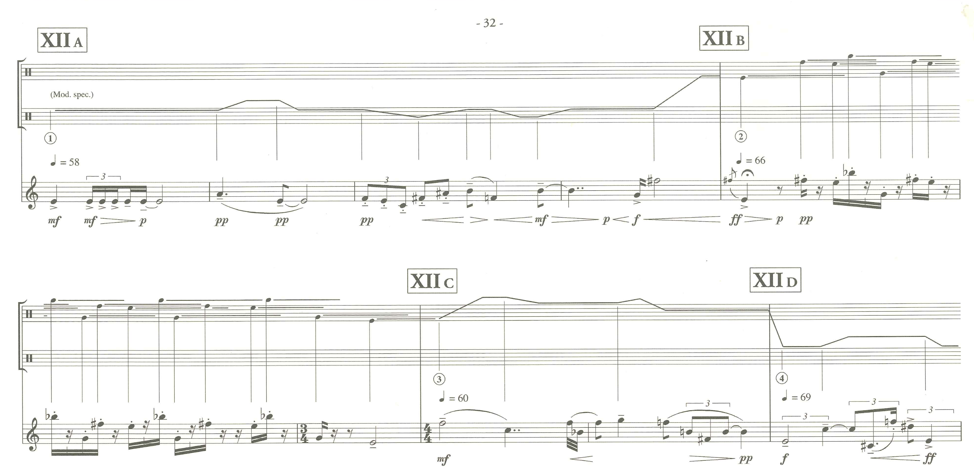
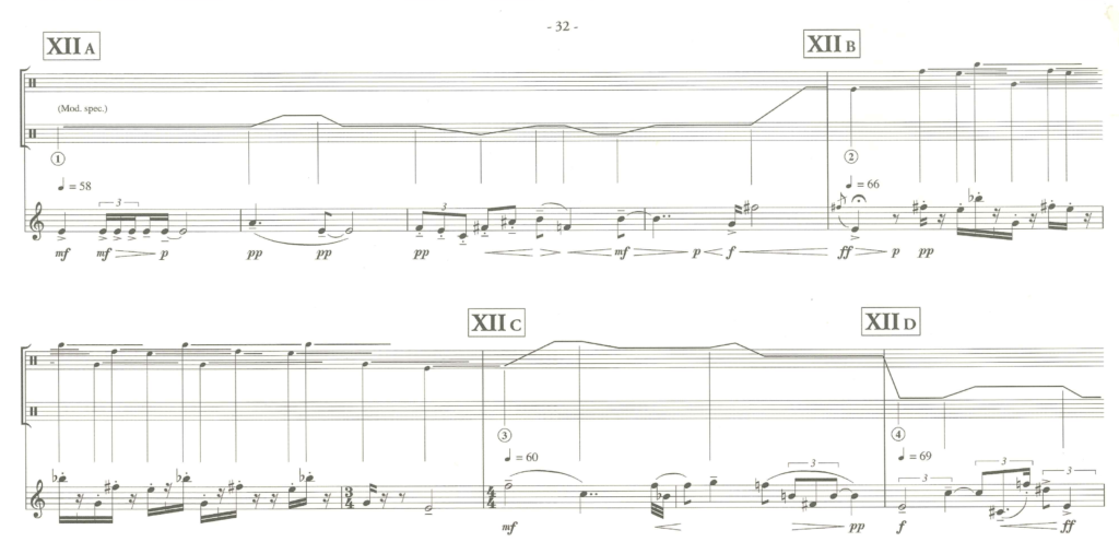
Let us look a bit deeper into Manoury’s masterpiece “Jupiter” (1987). Although this piece is an early example of the advanced use of electronics with a computer, the use of adaptive parameters was used actively. For a detailed analysis and explanation of the composition, refer to May (2006). In sections VI and XII the flutist’s playing influences the change of timbre over time. The attack of the flutist’s notes (called note-incipits in May, 2006) control the frequency of the 28 oscillators of the chapo synthesizer – a type of additive synthesis with spectral envelope (Ibid, p. 149) – and its filters. The score also shows these changes in timbre (and pitch) throughout the score (Manoury, 2008, p.32). This is around the 23:06 mark in the recording done my Elizabeth McNutt (2001).

Several other sections’ temporality is also influenced by the performer. For example, in section II, the computer will record short instances of the performer which only be used later in section V and IX in which these excerpts are interpolated and then morphed into tam-tam hits or piano. As May (2006) notes, the flutist’s line directly affects the shape, speed and direction of the interpolations marking a clear relationship between both parts. The sections in which the performer is recorded is clearly marked in the score. In several of the interpolation sections, the electronics take the lead and the performer is told to wait for certain musical elements. The score is also clear about how the interpolations are played and how they are directly related to the performer’s actions.

The composer Hans Tutschku has also used this idea in his series “Still Air” which currently features three compositions (2013, 2014, 2014). In all the pieces, the musicians are to play along to an iPad which might be easier than installing MaxMSP, a soundcard and external microphone for many musicians. The iPad’s built in microphone is used to measure the musicians’ amplitude which varies the amplitude and pitch of the playback files. The exact relationship between the musician and electronics vary throughout the composition. This means that the way the amplitude of the signal modifies the pitch and loudness of the playback part will vary depending on the current event number which are shown in the score (Tutschku, personal communication, October 10, 2017). This use of adaptive parameters is simple and still permits the composer to have a large influence between performer and computer.

A third and final example is “Mahler in Transgress” (2002-2003) by Flo Menezes, especially its restoration done in 2007 by Andre Perrotta which uses Kyma (Perrotta, personal communication, October 6, 2017). Parameters from both pianists are used to control several aspects of the electronics. For example, the sound of one piano could filter the other, or one’s amplitude could affect the spectral profile of the other. Throughout the duration of the composition, the electronics are mainly processing both pianos, as they influence their timbre between each other. This creates a clear relationship between what both performers are playing and the electronics that the audience can hear.

These are only three examples that this author believes shows many different possibilities for the use of adaptive parameters in through-composed music. It is by no means meant to be an exhaustive list, but only as a start to have a common language and understanding on adaptive parameters in mixed music.

A Composition Must Be Like the World or… ?

Gustav Mahler’s (perhaps apocryphal) citation “A symphony must be like the world. It must contain everything” is often popular with composition students. However, this author’s understanding of composition especially in the field of mixed music has led him to believe that a composition should be a world on its own. Its rules should be guided by the poetical meaning of the composition. The rules and ideas that will suit one composition’s electronics and structures, will not necessarily suit another composition. Each composition (its whole of the score and the computer program/electronics) forms its own world.

With this article, this author does not wish to delve into a debate over aesthetics. However, these concepts and possibilities tend to go towards music done in real-time. For years, it was thought that the possibilities of live electronics were limited, but in recent years this has not been the case. The field is still ripe with the possibilities of experimentation within the world of through-composed music.

At this point in time, this author is also experimenting directly with the concept of cross-adaptive synthesis written into through-composed music. I see no reasons as to why it shouldn’t be used both in and out of freely improvised music. We should think of technology and its concepts not within aesthetic boundaries, but as how we can use it for our own purposes.

Bibliography

Cont, A. (2008). “ANTESCOFO: Anticipatory synchronization and control of interactive parameters in computer music.” in Proceedings of international computer music conference (ICMC). Belfast, August 2008.

Frengel, M. (2010). A Multidimensional Approach to Relationships between Live and Non-live Sound Sources in Mixed Works. Organised Sound , 15 (2), 96–106. https://doi.org/10.1017/S1355771810000087

Manoury, P. (1997). Les partitions virtuelles in « La note et le son: Écits et entretiens 1981-1998 » . Paris, France: L’Harmattan.

Manoury, P. (1998). Jupiter (score, originally 1987, revised in 1992, 2008). Italy: Universal Music MGB Publishing.

Mcnutt, Elizabeth (2001). Pipewrench: flute & computer (Music recording). Emf Media.

May, Andre (2006). Philippe Manoury’s Jupiter. In Simoni, Mary (Ed.), in Analytical methods of electroacoustic music (pp. 145-186). New York, USA : Routledge Press.

Ramstrum, Momilani (2006). Philippe Manoury’s opera K…. In Simoni, Mary (Ed.), in Analytical methods of electroacoustic music (pp. 239-274). New York, USA : Routledge Press.

Session with 4 singers, Trondheim, August 2017

Location: NTNU, Studio Olavshallen.

Date: August 28 2017

Participants:
Sissel Vera Pettersen, vocals
Ingrid Lode, vocals
Heidi Skjerve, vocals
Tone Åse, vocals

Øyvind Brandtsegg, processing
Andreas Bergsland, observer and video documentation
Thomas Henriksen, sound engineer
Rune Hoemsnes, sound engineer

We also had the NTNU documentation team (Martin Kristoffersen and Ola Røed) making a separate video recording of the session.

Session objective and focus:
We wanted to try out crossadaptive processing with similar instruments. Until this session, we had usually used it on a combination of two different instruments, leading to very different analysis conditions. The analysis methods reponds a bit differently to each instrument type, and they also each “trigger” the processing in particular manner. It was thought interesting to try some experiments under more “even” conditions. Using four singers and combining them in different duo configurations, we also saw the potential for gleaming personal expressive differences and approaches to the crossadaptive performance situation. This also allowed them to switch roles, i.e. performing under the processing condition where they previously had the modulating role. No attempt was made to exhaustively try every possible combination of roles and effects, we just wanted to try a variety of scenarios possible with the current resources. The situation proved interesting in so many ways, and further exploration of this situation would be neccessary to probe further the research potential herein.
In addition to the analyzer-modulator variant of crossadaptive processing, we also did several takes of live convolution and streaming convolution . This session was the very first performative exploration of streaming convolution.

We used a reverb (Valhalla) on one of the signals, and a custom granular reverb (partikkelverb) on the other. The crossadaptive mappings was first designed so that each of the signals could have a “prolongation” effect (larger size for the reverb, more time smearing for the granular effect). However, after the first take, it seemed that the time smearing for the granular effect was not so clearly perceived as a musical gesture. We then replaced the time smearing parameter of the granular effect with a “graininess” parameter (controlling grain duration). This setting was used for the remaining takes. We used transient density combined with amplitude to control the reverb size, where louder and faster singing would make the reverb shorter (smaller). We used dynamic range to control the time smearing parameter of the granular effect, and used transient density to control the grain size (faster singing makes the grains shorter).

Video digest of the session

Crossadaptive analyzer-modulator takes


Crossadaptive take 1: Heidi/Ingrid
Heidi has a reverb controlled by Ingrids amplitude and transient density
– louder and faster singing makes the reverb shorter
Ingrid has a time smearing effect.
– time is more slowed down when Heidi use a larger dynamic range


Crossadaptive take 2: Heidi/Sissel
Heidi has a reverb controlled by Sissels amplitude and transient density
– louder and faster singing makes the reverb shorter
Sissel has a granular effect.
– the effect is more grainy (shorter grain duration) when Heidi play with a higher transient density (faster)


Crossadaptive take 3: Sissel/Tone
Sissel has a reverb controlled by Tones amplitude and transient density
– louder and faster singing makes the reverb shorter
Tone has a granular effect.
– the effect is more grainy (shorter grain duration) when Sissel play with a higher transient density (faster)


Crossadaptive take 4: Tone/Ingrid
Ingrid has a reverb controlled by Tones amplitude and transient density
– louder and faster singing makes the reverb shorter
Tone has a granular effect.
– the effect is more grainy (shorter grain duration) when Ingrid play with a higher transient density (faster)


Crossadaptive take 5: Tone/Ingrid
Same settings as for take 4

Convolution

Doing live convolution with two singers was thought interesting for the same reasons as listed in the introduction, creating a controlled scenario with two similarly-featured signals. As vocal is in itself one of the richest instruments in terms of signal variation, it was also intersting to explore convolution wwith these instruments. We used the now familiar live convolution techniques, where one of the performers record an impulse response and the other plays through it. In addition, we explored streaming convolution , developed by Victor Lazzarini as part of this project. In streaming convolution, the two signals are treated even more equally that what is the case in live convolution. Streaming convolution simply convolves two circular buffers of a predetermined length, allowing both signals to have the exact same role in relation to the other. It also has a “freeze mode”, where updating of the buffer is suspended, allowing one or the other (or both) of the signals to be kept stationary as a filter for the other. This freezing was controlled by a physical pedal, in the same manner as we use a pedal to control IR sampling with live convolution. In some of the videos one can see the singers raising their hand, as a signal to the other that they are now freezing their filter. When the signal is not frozen (i.e. streaming), there is a practically indeterminate latency in the process as seen from the performer’s perspective. This stems from the fact that the input stream is segmented with respect to the filter length. Any feature recorded into the filter will have a position in the filter dependent on when it was recorded, and the perceived latency between an input impulse and the convolver output of course relies on where in the “impulse response” the most significant energy or transient can be found. The techical latency of the filter is still very low, but the perceived latency depends on the material.


Liveconvolver take 1: Tone/Sissel
Tone records the IR


Liveconvolver take 2: Tone/Sissel
Sissel records the IR


Liveconvolver take 3: Heidi/Sissel
Sissel records the IR


Liveconvolver take 4: Heidi/Sissel
Heidi records the IR


Liveconvolver take 5: Heidi/Ingrid
Heidi records the IR

Streaming Convolution

These are the very first performative explorations of the streaming convolution technique.


Streaming convolution take 1: Heidi/Sissel


Streaming convolution take 2: Heidi/Tone