Location: Studio Olavskvartalet , NTNU, Trondheim
Participants:
Trond Engum, Andreas Bergsland, Tone Åse, Thomas Henriksen, Oddbjørn Sponås, Hogne Kleiberg, Martin Miguel Almagro, Oddbjørn Sponås, Simen Bjørkhaug, Ola Djupvik, Sondre Ferstad, Björn Petersson, Emilie Wilhelmine Smestad, David Anderson, Ragnhild Fangel
Session objective and focus:
This post is a description of a session with 3rd year Jazz students at NTNU. It was the first session following the intended procedure framework for documentation of sound and video in the cross adaptive processing project. The session was organized as part of the ensemble teaching that is given to Jazz students at NTNU, and was meant to take care of both the learning outcomes from the normal ensemble teaching, and also aspects related to the cross adaptive project. This first approach was meant as a pilot for the processing musician and the video and documentation aspect. It can also be seen as a test on how musicians not directly involved in the project react and reflect within the context of cross adaptive processing. We made a choice to keep the processing system as simple as possible to make the technical aspect of the session as understandable as possible for all parts involved. To achieve this we only used analyses of RMS and transient density on the instruments to link conventional instrumental performance close to how the effects were controlled. As an example: The louder you play either the more or less of one effect is heard, or depending on the transient density the more or less of one effect is heard. All instruments were set up to control the amount of processed signal on two different effects each, giving the system a potential to use up to four different effects at the same time. The processing musician had a possibility to adjust the balance between the different processed signals during performance. The direct signal from the instruments was also kept as part of the mix to reduce an alienation from the acoustic sound of the instrument since this was a first attempt for those involved. Since the musicians, besides performing on their instruments, also indirectly perform the sound production we chose to follow up a premise of a shared listening strategy used by the T-Emp ensemble. https://www.researchcatalogue.net/view/48123/53026 The basic idea is that if everyone hears the same mix, they will adjust individually and consequently globally to the sound image as a whole through their instrumental and sound production output.
Sound examples:
Besides normalising, all sound examples presented in this post are unprocessed and unedited in postproduction meaning that they have the same mix between instruments and processing as the musicians and observers auditioned during recording.
20.09.2016
Take 1 – Session 20.09.16 take 1 drums_piano.wav
Drums and piano
Drums controlling the volume of how much overdrive or reverb is added to the piano. The analysing parameters used on the drums are rms_dB and trans_dens. The louder the drums play, the more overdrive on the piano, and the larger transient density the less reverb on the piano. The take has some issues with bleeding between microphones since both performers are in the same room. There was also a need for fine-tuning the behaviour of both effects through the rise and fall parameters in the mediator plug in during the take.
Even though it would be natural to presume that more is more in a musical interplay – for example that the louder you play the more effect you receive – the performers experienced that more is less was more convenient on the reverb in this particular setting. It felt natural for the musicians that when the drummer played faster (higher degree of transient density) the amount of reverb on the piano was decreased. After this take we had a system crash. As a consequence the whole set up was lost, and a new set up was built from scratch for the rest of the session.
Take 2 – Session 20.09.16 take 2 drums_piano.wav
Drums and piano
The piano controlling the loudness on the amount of echo and reverb are added to the drums. The larger transient density the more echo on drums, the louder piano the more reverb on the drums.
Take 3 – Session 20.09.16 take 3 drums_piano.wav
The piano controlling the volume of how much echo and reverb are added to the drums. The larger transient density the more echo on drums, the louder piano the more reverb on the drums. Loudness on drums controls overdrive on piano (the louder the more overdrive), and transient density controls reverb – the larger transient density the less reverb on the piano.
21.09.2016
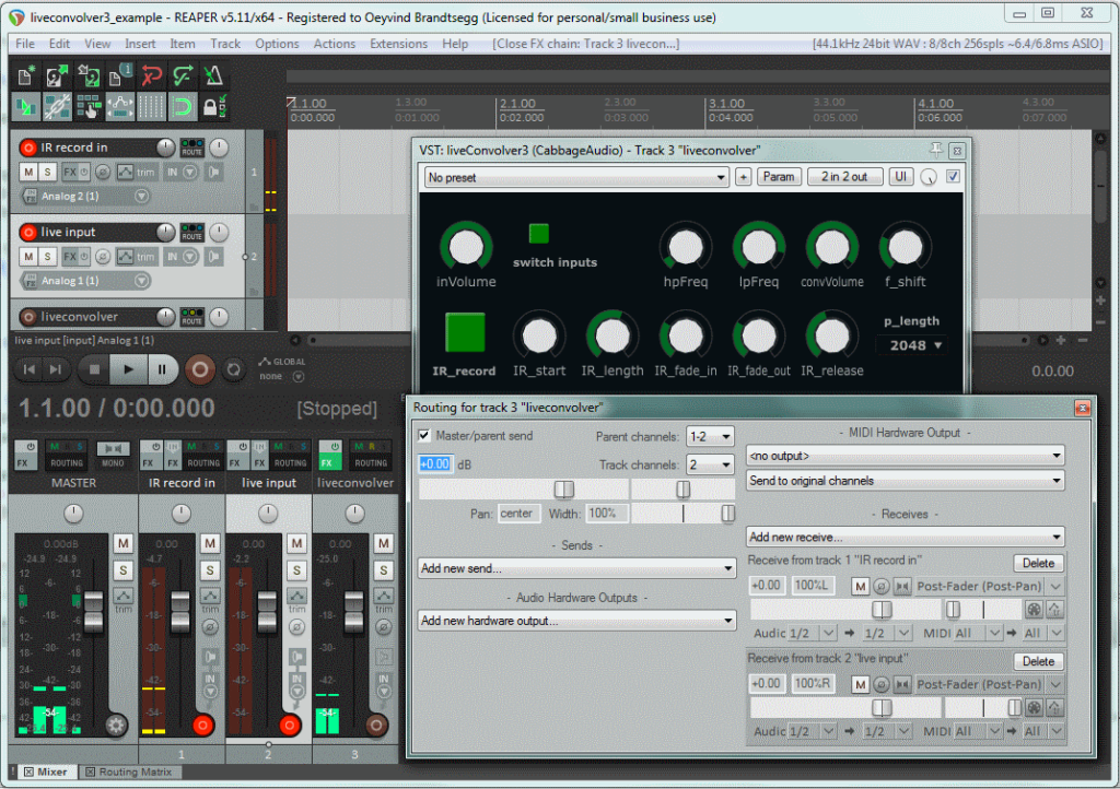
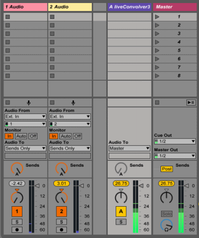
Due to technical challenges the first day we made some adjustments on the system in order to avoid the most obvious obstacles. We changed from condenser to dynamic microphones to decrease the amount of bleeding between them (bleeding affects the analyser plug-in and also adds the same effect to both instruments, as experienced earlier in the project). The reason for the system crash was identified in the Reaper setup, and a new template was also made in Ableton live. We chose to keep the set up simple during the session to clarify the musical results (Only two analysing parameters controlling two different effects on each instrument).
Take 1 – Session 21.09.16 take 1 drums_guitar.wav
Percussion and guitar
Percussion controlled the amount of effect on the guitar using rms-dB and trans-dens as analysis parameters – the louder percussion, the more reverb on the guitar, and the larger the transient density on percussion, the more echo on the guitar. This set up was experienced as uncomfortable for the performers, especially when loud playing resulted in more reverb. There was still an issue with bleeding even though we had changed to dynamical microphones.
Take 2 – Session 21.09.16 take 2 drums_guitar.wav
We agreed upon some changes suggested by the musicians. We used the same analysis parameters on the percussion, with percussion controlling the amount of effect on the guitar, using rms-dB and trans-dens: The louder percussion, the less overdrive on guitar, and the larger transient density of the percussion, the more echo on guitar. This resulted in a more comfortable relationship between the instruments and effects seen from the performers perspective.
Take 3 – Session 21.09.16 take 3 drums_guitar.wav
This setup was constructed to interact both ways through the effects applied to the instruments. We used the same analysis parameters on the percussion with percussion controlling the amount of effect on the guitar, using rms-dB and trans-dens: The louder percussion, the less overdrive on guitar, and the more transient density of the percussion, the more echo on guitar. We used the same analysis parameters on the guitar as on the percussion (rms-dB and trans-dens): The louder guitar, the more overdrive on percussion, and larger transient density on guitar the more reverb on percussion. During this session the percussionist also experimented with the distance to the microphones to test out movement and proximity effect in connection with the effects. The trans-dens analyses on the guitar did not work as dynamically as expected due to some technical issues during the take.
Take 4 – Session 21.09.16 take 4 harmonica_bass.wav
Double bass and harmonica
We started out with letting the harmonica control the effects on the double bass based using the analyses of rms-dB and trans_dens. The more harmonica volume, the less overdrive on bass, and the more transient density on the harmonica, the more echo on bass. This first take was not very successful due to bleeding between microphones (dynamical). There was also an issue with the fine-tuning in the mediator concerning the dynamical range sent to the effects. This resulted in a experience that the effects where turned on and off, and not changed dynamically over time which was the original intention. There was also a contradiction between musical intention and effects. (The harmonica playing louder reducing overdrive on the bass)
Take 5 – Session 21.09.16 take 5 harmonica_bass.wav
Based on suggestions by the musicians we set up a system controlling effects both ways. The harmonica still controlled the effects on the double bass based on the analyses of rms-dB and trans_dens, but now we tried the following: The more harmonica volume, the more overdrive on bass, and the more transient density, the more echo on bass. The bass used analyses of two instances of rms-dB to control the effects on the harmonica: The louder the bass, the less reverb on the harmonica, and the louder the bass the more overdrive on the harmonica. This set created a much more “intuitive” musical approach seen from the performers perspective. The function with the harmonica controlling the bass overdrive worked against the performers musical intention, and this functionality was removed during the take. This should probably not have been done during a take, but it was experienced as a bit confusing for the instrumentalists in this setting. This take show how dependent the musicians are on each other in order to “activate” the effects, and also the relationship and potential between musical energy followed up by effects.
Take 6 – Session 21.09.16 take 6 vocals_saxophone.wav
Vocals and Saxophone
In this setup the saxophone controls the effects on the vocals based on two instances of rms_dB analyses: The louder the saxophone, the less reverb on the vocals, and the louder the saxophone, the more echo is added to the vocals. The first attempt had some problems with the balance between dry and wet signal in the mix from the control room. The vocal input was lower compared to sources present earlier that day. As a consequence, the saxophone player was unable to hear both the direct signal of the voice, but also the effects he added to the voice. This was tried compensated for during the take by boosting the volume of the echo during the take, but without any noticeable result in the performance. Another challenge that occurred in this take was a result of the choice of effects. Both reverb and echo can sound quit similar on long vocal notes, and as a consequence blurred the experienced amount of control over the effects. This pinpoints the importance of good listening conditions for the musicians in this project, especially if working with more subtle changes in the effects.
Take 7 – Session 21.09.16 take 7 vocals_saxophone.wav
Before recording a new take we made adjustments in the balance between wet and dry sound in the control room. We then did a second take with the same settings as take 6. It was clear that the performers took more control over the situation because of better listening conditions. The performers expressed a wish to practise with the set up on beforehand. Another aspect that was asked for by the performers was that the system should open up for subtle changes in the effects while still keeping the potential to be more radical at the same time depending on the instrumental input. The saxophone player also mentioned that it could be interesting to add harmonies as one of the effects since both instruments are monophonic.
Take 8 – Session 21.09.16 take 8 vocals_saxophone.wav
The last take of the day included the vocals to control the effects on the saxophone. The saxophone was kept with the same system as in the two former takes: The louder the saxophone, the less reverb on the vocals, and the louder the saxophone, the more echo was added to the vocals. The vocals were analysed by rms_dB and trans_dens: The more loudness on vocals, the more overdrive on saxophone, and the larger transient density on the vocals, the more echo on the saxophone. Both performers experienced that this system was meaningful both musically and in aspect of control over the effects. They communicated that there was a clear connection between the musical intention and the sounding result.
Comments:
All the involved musicians communicated that the experiment was meaningful even though it was another way of interacting in a musical interplay. The performers want to try this more with other set ups and effects. Even though this was the first attempt for the performers and the processing musician we achieved some promising musical results.
Technical issues to be solved:
- There are still some technical issues to be solved in the software (first of all avoiding system crashes during sessions). Bleeding between microphones is also an issue that needs to be attended to. (This challenge will be further magnified in a live setting).
- On/off control versus dynamical control, We need more time together with the performers to rehearse and fine – tune the effects.
- Performers involved need more time together with the processing musician to rehearse before takes in order to familiarize with the effects and how they affect them.
- The performers experience of being in control/not being in control of the effects.
Other thoughts from the performers:
- Suggestions about visual feedback and possibility to make adjustments directly on the effects themselves.
- It could be interesting to focus just as much on removing attributes from the effects through instrumental control as adding. (Adding more effects is often the first choice when working with live electronics.
- Agree upon an aesthetical framework before setting up the system involving all performers.
Link to a video with highlights from the session: