
Many of the currently used methods for rhythmic analysis, e.g. in MIR, makes assumptions about musical style, and for this reason does particularly well in analysing music within certain geographical and/or cultural origins. For our purposes we’d rather try to find analysis methods of a more generic nature. We want our analysis methods to be adaptable to many different musical situations. Also, since we assume the performance can be of an improvised nature, we do not know what is going to be played before it is actually performed. Finally, the audio stream to be analyzed is a realtime stream and this poses certain restrictions as we can not for example do multiple passes iterating over the whole song.
A goal at this point has been to try to find methods of rhythmical analysis that work without assumptions about pulse and meter. One such methods could be based just on the immediate rhythmic ratios between adjacent time intervals. Our basic assumption is then that rhythm consists of time intervals, and the relationship between these intervals. As such we can describe rhythm as time ratio constellations, patterns of time ratios. Moreover, simple rhythms are created from simple ratios, more complex rhythms from more irrational and irrregular combinations of time intervals. This could give rise to a measurement of some kind of rhythmic complexity, although rhythmic complexity may be made up of complexity in many different dimensions, so we need to come back to what we actually will use as a term for the output of our analyses. Then, sticking to complexity for the time being, how do we measure the complexity of the time ratios?
One way of looking at the time ratios (also grouping them into cathegories) is to represent them as the closest rational approximation. Using the
Farey sequence
, we can find the closest rational approximation with a given highest denominator. For example, a ratio of 0.6/1 will be approximated by 1/2 (1/2 = 0.5) , 2/3 (= 0.667), or 3/5 (= 0.6 exactly) depending on how high we allow the denominator to go. This way, we can decide how finely spaced we want our rhythm analysis grid to be. In the previous example, if we decided not to go higher than 3 for the denominator, we would only roughly approximate the actual observed time ratio but in return always get relatively simple fractions to work with. Deciding on an appropriate grid can be difficult, since the allowed deviation by human musical perception will often be higher even than the difference between relatively simple fractions (for example in the case of an extreme ritardando or other expressive timing). The
perceived rhythm
also being dictated by musical context. As the definition (or assertion) of musical context always will make assumptions about musical style, our current rhythmic analysis method does not take a larger musical context into account. We will however make a small
local rhythmic context
out of groupings of time ratios that follow each other. The current implementation includes 3 time ratios, so it effectively considers rhythmic patterns of up to 4 events as a rhythmic motif to be analyzed. This also allows it to respond quickly to changes in the performed rhythm, as it will only take 2 events of a new rhythmic pattern to generate a significant change in the output. This relative simplicity may also help us in narrowing down the available choices to making up a rhythmic grid for the approximations. If we regard only separate time ratios between neighbouring events, there are some ratios that will be more likely than others. Halving and doubling of tempo, tripling etc obviously will happen a lot, and more so, they will happen a lot more that what you’d expect. Say for example the rhythmic pattern of steady quarter notes followed by some steady 8th notes, then back to quarter notes:
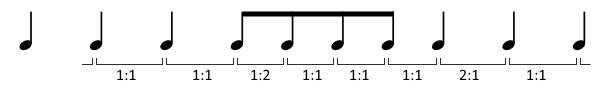
Here, we will observe the ratio of 1/1 between the quarter notes, then the ratio 2/1 when we change into 8th notes, and then 1/1 for as long as we play 8th notes, and a ratio of 1/2 when we move back to quarter notes. Similarly for triplets, except we’d go 1/1, 3/1, 1/1, 1/3, 1/1.
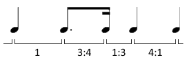
Certain common rhythmic patterns (like a dotted 8th followed by a 16th) may create 3/4 and 1/3 ratios.
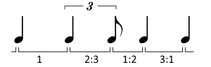
or with triplets, 2/3 and 1/2 ratios:
See, all these ratios express the most recent time interval as a ratio to the next most recent one. More complex relationships are also of course observed quite commonly. We have tried to describe ratios assumed to be more frequently used. The list of ratios at the time of writing is [1/16, 1/8, 1/7, 1/6, 1/5, 1/4, 1/3, 1/2, 3/5, 2/3, 3/4, 1/1] for ratios below 1.0, and then further [5/4, 4/3, 3/2, 5/3, 7/4, 2/1, 3/1, 4/1, 5/1, 6,/1, 7/1, 8/1, 12/1, 16/1]. The selection of time ratios to be included can obviously be the focus of a more in-depth study. Such a study could analyse a large body of notated/composed/performed patterns in a wide variety of styles to find common ratios not included in our initial assumptions (and as an excercise to the reader: find rhythms not covered by these ratios and send them to us). Analysis of folk music and other oral musical traditions, radical interpretations and contemporary music will probably reveal time ratios currently not taken into account by our analysis. However, an occational missed ratio will perhaps not be a disaster to the outputof the algorithm. The initial template of ratios let us get started, and we expect that the practical use of the algorithm in the context of our cross-adaptive purposes will be the best test for its utility and applicability. The current implementation use a lookup table for the allowed ratios. This was done to make it easier to selectively allow some time ratios while excluding others of the same denominator, for example allowing 1/16 but not 15/16. Again, it migh be a false assumption that the music will not contain the 15/16 ratio, but as of now we assume it is then more likely that the intended ratio was 16/16 boiling down to 1/1).
Rhythmic consonance
So what can we get out of analysing the time ratios expressed as simple fractions? A basic idea is that simpler ratios represent simpler relationships. But how do we range them? Is 3/4 simpler than 2/3? Is 5/3 simpler than 2/7? If we assume rhythmic ratios to be in some way related to harmonic ratios, we can find theories within the field of just intonation and microtonality, where the Benedetti height (the product of the numerator and denominator) or Tenney height (log of the Benedetti height) is used as a measure of inharmonicity. For our purpose we multiply the normalized Tenney height (with a small offset to avoid zeros for log(0)), of the three latest time intervals, as this will also help short term repetitions to show up as low inharmonicity. So if we take the inverse of inharmonicity as a measure of consonance, we can in the context of this algorithm invent the term “rhythmic consonance” and use it to describe the complexity of the time ratio.
Rhythmic irregularity
Another measure of rhythmic complexity might be the plain irregularity of the time intervals. So for example if all intervals have a 1/1 ratio, the irregularity is low because the rhythm is completely regular. Gradual deviations from the steady pulse give gradually higher irregularity. For example a whole note followed by a 16th note (16/1) is quite far from the 1/1 ratio so this yields a high irregularity measure. As a means of filtering out noise (for example due to single misplaced events), we take the highest two out of the last three irregularity measurements, then we multiply them with each other. In addition to acting like a filter, it also provides aa little more context than just measuring single events. Finally the resulting value is lowpass filtered.
Deviation
In our quantization of time intervals into fractions we may sometimes have misinterpreted the actual intended rhythm, as described above. Although we have no measure of how far the analyzed fraction is from the
musically intended
rhythm, we can measure how far the observed time interval is from the quantized one. We can call this
rhythm ratio deviation
, and it is expressed as a fraction of the interval between possible quantizations. For example if our quantization grid consist of 1/4, 1/3, 1/2, 2/3, 3/4 and 1/1 (just for the case of the example), and we observe a time ratio of 0.3, this will be expressed as 1/3 in the rhythmic ratio analysis since that is the ratio it is closest to. To express the deviation between the observed value and the quantized value in a practically usable manner, we need to scale the numeric deviation by the interval within which it can deviate before being interpreted as some other fraction. Lets number the fractions in our grid as
, that is, the first fraction is
,the second is
, and so on. We call the actual observed time ratio
and the quantized time ratio
. The deviation can then be expressed as
in our case. If the observed ratio was rounded down when quantizing, the formula would use
in place of
:
The deviation measure is not reasonably used for anything musical as a control signal, but it can give an indication of the quality of our analysis.
The GUI
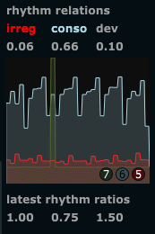
For the display of the rhythm ratio analysis, we write each value to a cyclic graph. This way one can get an impression of the recent history of values. There is a marker (green) showing the current write point, which wraps around when it reach the end. Rhythm consonance values are plotted in light blue/grey, rhythm irrregularity is plotted in red. The deviation and the most recent rhythm ratios are not plotted but just shown as number boxes updated on each rhythmic event.
Next up
Next post on rhythmic analysis will be looking at patterns on a somewhat longer time scale (a few seconds). For that, we’ll use autocorrelation to find periodicities in the envelope.