As we started the project, Oeyvind and myself were discussing a few things we thought should be added directly to Csound in order to allow more efficient signal analysis. The first of these things we looked at were components to allow Mel Frequency Cepstral Coefficients (MFCCs) to be calculated.
We have already various operations on arrays, to which I thought could we could add other things, so that we have all the components necessary for MFCC computation. The operations we need for MFCCs are:
– windowed Discrete Fourier Transform (DFT)
– power spectrum
– Mel-frequency filterbank
– log
– Discrete Cosine Transform (DCT)
Window -> DFT -> power spectrum -> MFB -> log -> DCT -> MFCCs
Of these, we had everything in place but the filterbank and the DCT. So I went off to add these two operations. I’ll spend some time in this post discussing some features of the DCT and the process of implementing it.
The DCT is one of these operations a lot of people use but do not understand it well. The earliest mention I see of it in the literature is on a paper by Ahmed, Natarajan and Rao, “ Discrete Cosine Transform ” , where one of its forms (the type-II DCT) and its inverse are presented. Of course, the idea originates from the so-called half-transforms, which include the continuous-time, continuous-frequency Cosine Transform and the Sine Transform, but here we have a fully discrete-time discrete-frequency operation.
In general, we would expect that a transform whose bases are made up of cosines would correctly pick up on cosine-phase components of a signal and so does the DCT. However, this is only part of the history, because implied in this is that a signal will be modelled by cosines, so that what we are trying to do is to think of this as a periodically repeated function with even boundaries (“symmetric” or “mirror-like”). In other words, that its continuation beyond the particular analysis window is modelled as even. The DFT, for instance, does not assume this particular condition, but only models the signal as a single cycle of a waveform (with the assumption that it is repeated periodically).
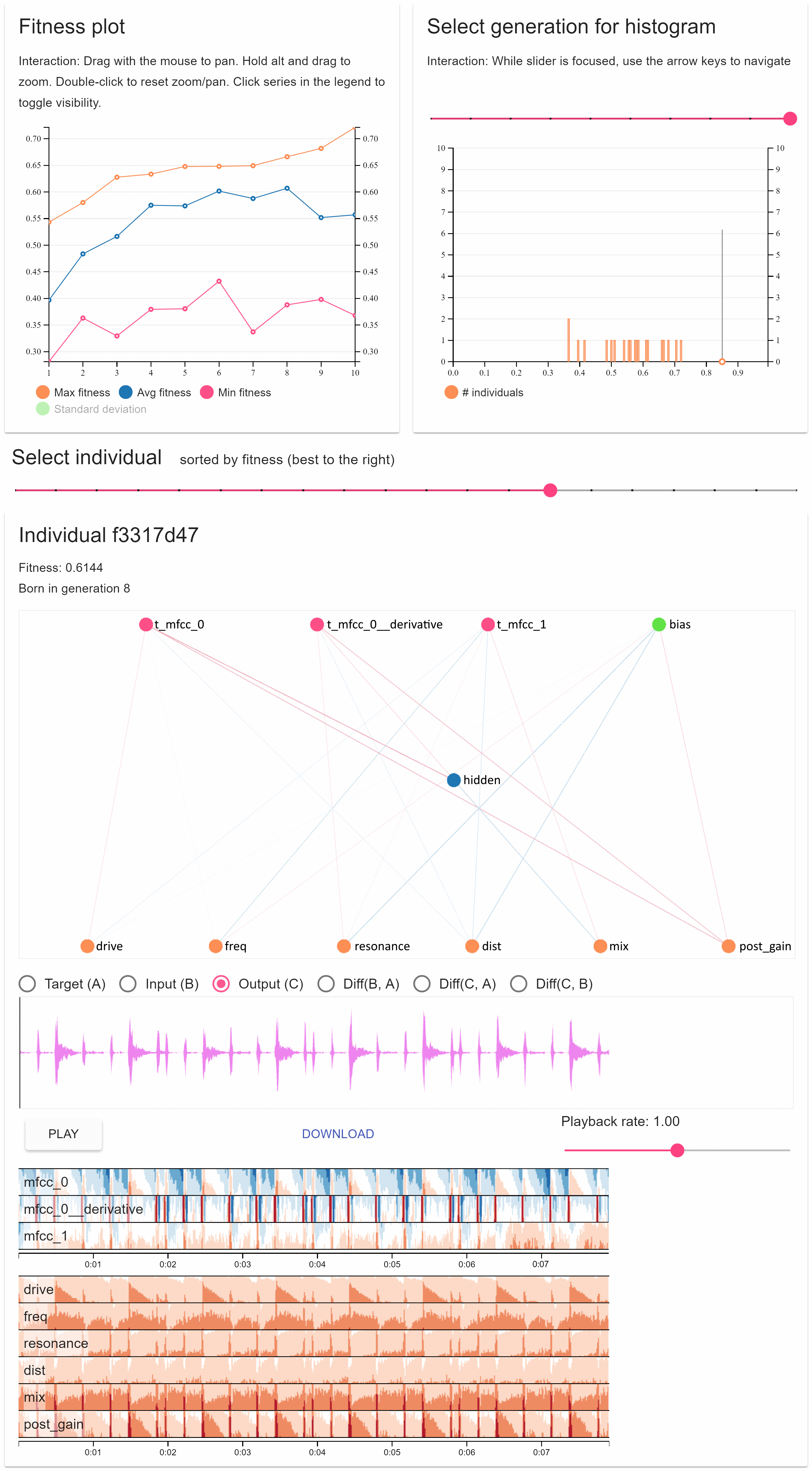
This assumption of evenness is very important. It means that we expect something of the waveform in order to model it cleanly, but that might not always be possible. Let’s think of two cases: cosine and sine waves. If we take a DFT and its magnitude spectrum of one full cycle of these functions, we will detect a component in bin 1 in both cases, as expected
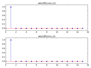
With DCT, however, because it assumes even boundaries, we only get a clean analysis of the cosine wave (because it is even), whereas the sine (which is odd) gets smeared all over the lower-order bins:
Note also that in the cosine case, the component is picked up by bin 2 (instead of bin 1). This can be explained by the fact that the series used by the DCT is based on multiples of a 1/2-cycle cosine (see the expression for the transform below) and so a full-period wave is actually detected in the second analysis frequency point.
So the analysis is not particularly great in the case of non-symmetric inputs, but it actually does what it says on the tin: it models the signal as if it were made of a sum of cosines. The data can also be inverted back to the time domain, so we can recover the original signal. Despite these conditions, the DCT is used in many applications where its characteristics are appropriately useful. One of these is in the computation of the MFCCs as outlined above, because in this process we are using the power spectrum (split into a smaller number of bands by the MFB) as the input to the DCT. Since audio signals are real-valued, this is an even function and so we can model it very well with this transform.
In the case of the DCT II, which we will be implementing, the signal is assumed to be even at both the start and end boundaries. In addition, the point of symmetry is placed halfway between the first signal sample and its implied predecessor, and halfway between the last sample and its implied successor. This also implies a half-sample delay in the input signal, something that is clearly seen in the expression for the transform:

Finally, when we come to implement it, there are two options. If we have a DCT available in one of the libraries we are using, we can just employ it directly. In the case of Csound, this is only available in one of the platforms (OSX through the accelerate framework) and so we have to use our second option: re-arrange the input data and apply it to a real-signal DFT.
The DCT II is equivalent (disregarding scaling) to a DFT of 4N real inputs, where we re-order the input data as follows:

where y(n) is the input to the DFT and x(n) is the input to the DCT. You can see that all even-index samples are 0 and the input data is placed in the odd samples, symmetrically about the centre of the frame. For instance if the DCT input is [1,2,3,4], the DFT input will be [0,1,0,2,0,3,0,4,0,4,0,3,0,2,0,1]. Once this re-arrangement is done, we can take the DFT and then scale it by 1/2.
For this purpose, I added a couple of new functions to the Csound code base, to perform the DCT as outlined above and its inverse operation. These use the new facility where the user can select the underlying FFT implementation, either the original fftlib, PFFFT, or accellerate (veclib, OSX and iOS only) via an engine option. To make this available in the Csound language, two new array operations were added:
i/kOut[] dct i/kSig[] and i/kOut idct i/kSpec[]
With these, we are able to code the final step in the MFCC process. In my next blogpost , I will discuss the implementation of the Mel-frequency filterbank, which completes the set of operators needed for this algorithm.