Oeyvind

As preparation for upcoming discussions about tecnical needs in the project, it seems appropriate to briefly describe the current status of the software developed so far.

The plugins

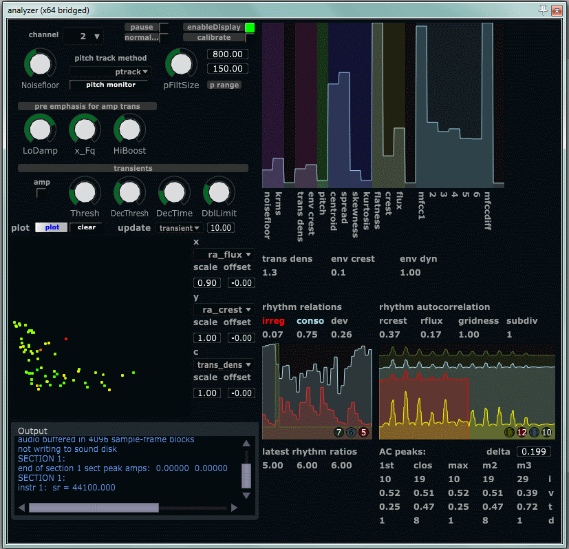
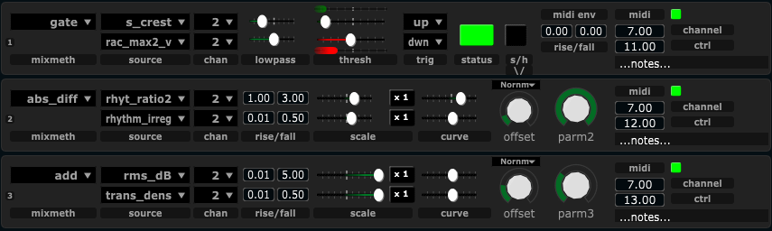
The two main plugins developed is the Analyzer and the MIDIator. The Analyzer extracts perceptual features from a live audio signal and transmit signals representing these features over a network protocol (OSC) to the MIDIator. The job of the MIDIator is to combine different analyzed features (scaling, shaping, mixing, gating) into a controller signal that we will ultimately use to control some effect parameter. The MIDIator can run on a different track in the same DAW, it can run on another DAW, or on another computer entirely.

Strong points

The feature extraction generally works reasonably well for the signals it has been tested on. Since a limited set of signals is readily available during implementation, some overfitting to these signals can be expected. Still, a large set of features is extracted, and these have been selected and tweaked for use as intentional musical controllers . This can sometimes differ from the more pure mathematical and analytical descriptions of a signal. The quality of of our feature extraction can best be measured in how well a musician can utilize it to intentionallly control the output. No quantitative mesurement of that sort have been done so far. The MIDIator contains a selection of methods to shape and filter the signals, and to combine them in different ways. Until recently, the only way to combine signals (features) was by adding them together. As of the past two weeks, mix methods for absolute difference, gating, and sample/hold has been added.

midiator_modules_2016_10 — MIDIator modules

Weak points

The signal chain transmission from Analyzer to MIDIator, and then again from the MIDIator to the control signal destination each incurs at least one sample block latency. The size of a sample block can vary from system to system, but regardless of the size used our system will have 3 times this latency before an effect parameter value changes in response to a change in the audio input. For many types of parameter changes this is not critical, still it is a notable limitation of the system.

The signal transmission latency points at another general problem, interfacing between technologies. Each time we transfer signals from one paradigm to another we have the potential for degraded performance, less stability and/or added latency. In our system the interface from the DAW to our plugins will incur a sample block of latency, the interface between Csound and Python can sometimes incure performance penalties if large chunks of data needs to be transmitted from one to the other. Likewise, the communication between the Analyzer and MIDIator is such an interface.

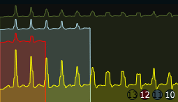
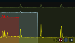
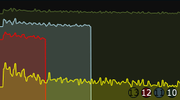
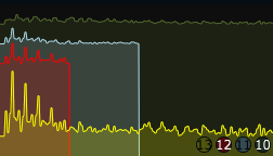
Some (many) of the feature extraction methods create somewhat noisy signals. With noise, we mean here that the analyzer output can intermittently deviate from the value we perceptually assume to be “correct”. We can also look at this deviation statistically, if we feed it relatively (perceptually) consistent signals and look at how stable the output of each feature extraction method is. Many of the features show activity generally in the right register, and a statistical average of the output corresponds with general perceptual features. While the average values are good, we will oftentimes see spurious values with relatively high deviation from the general trend. From this, we can assume that the feature extraction model generally works, but intermittently fails. Sometimes, filtering is used as an inherent part of the analysis method, and in all cases, the MIDIator has a moving exponential average filter with separate rise and fall times. Filtering can be used to cover up the problem, but better analysis methods would give us more precise and faster response from the system.

Audio separation between instruments can sometimes be poor. In the studio, we can isolate each musician, but if we want them to be able to play together naturally in the same room, a significant bleed from one instrument to the other will occur. For live performance this situation is obviously even worse. The bleed give rise to two kinds of problems: Signal analysis is disturbed by the signal bleed, and signal processing is cluttered. For the analysis, it does not matter if we had perfect analysis methods if the signal to be analyzed is a messy combination of opposing perceptual dimensions. For the effect processing, controlling an effect parameter for one instrument leads to a change in the processing of the other instrument, just because the other instruments’ sound bleed into the first instrument’s microphones

Useful parameters (features extracted)

In many of the sessions up until now, the most used features has been amplitude (rms) and transient density. One reson for this is probably that they are concptually easy to understand, another is that their output is relatively stable and predictable in relation to the perceptual quality of the sound analyzed. Here are some suggestions of other parameters that expectedly can be utilized effectively in the current implementation:

envelope crest ( env_crest ): the peakyness of the amplitude envelope, for sustained sounds this will be low, for percussive onsets with silence between evens it will be high
envelope dynamic range ( env_dyn ): goes low for signals operating at a stable dynamic level, high for signals with a high degree of dynamic variation.
pitch: well known
spectral crest ( s_crest) : goes low for tonal sounds, medium for pressed tones, high for noisy sounds.
spectral flux ( s_flux ): goes high for noisy sounds, low for tonal sounds
mfccdiff: measure of tension or pressedness, described here

There is also another group of extracted features that is potentially useful but still has some stability issues

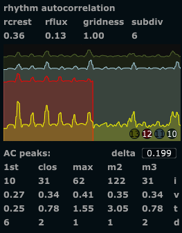
rhythmic consonance ( rhythm_cons ) and rhythmic irregularity ( rhythm_irreg ): described here
rhythm autocorr crest ( ra_crest ) and rhythm autocorr flux ( ra_flux ): described here

The rest of the extracted features can be considered more experimental, in some cases they might yield effective controllers, especially when combined with other features in reasonable proportions

As mentioned in the rhythm analysis part 1 , one of our goals at this point has been to try to find methods of rhythmical analysis that work without assumptions about pulse and meter, and also as far as possible without assumptions about musical style. As our somewhat minimal rhythm definition we look at rhythm as time ratio constellations , patterns of time ratios . Here we will make an assumption (yes, something must be assumed) regarding patterns of time durations: Recurring or repeated patterns have another perceptual quality than constantly shifting combinations of time durations. We could also assume that recurring or repeated patterns have stronger perceptual influence, but technically, it does not matter so much. The main issue is that we can measure some difference in quality. Quality here does not imply that something is better, just that something is different.

FFT of modified amplitude envelope

To measure how much recurrence there is in a signal, we can use autocorrelation. Repeated patterns will show up as peaks in the autocorrelation, and the period of repetition will be shown as the position of the peaks. Longer repetition periods give peaks further away (commonly further to the right when graphing the autocorrelation). To calculate the autocorrelation, we could use the FFT of the amplitude envelope as our basis. However, the unmodified envelope can have many variations at frequencies not related to the actual rhythms. For example, the amplitude envelope of a signal with fast transients (e.g. percussion, piano) show much more high frequency content than a signal with slow transients (e.g. many wind instruments). For this reason, we opted to use a modified envelope for the FFT in connection with the rhythm autocorrelation measure. The modified envelope is generated by using transient detection, triggering a short gaussian envelope scaled to the current amplitude of the signal. This way, we achieve a consistent envelope across different instruments, preserving the relative amplitude differences between transients (since we assume dynamics to be relevant to rhythm, for example in using accents to signify grouping of events).

Time spans and latency

One question to ask when analyzing for recurring patterns is “how long patterns are we looking for?” . One could say that a musical pattern sometimes will repeat relatively quickly, say once every second. Other times we can have arbitrary long patterns (sometimes very long), but for practical purposes, lets assume a maximum length of somewhere around 10 seconds. Now, if we want to analyze for such long patterns (10 seconds), an inherent limitation of any technique used would imply that it takes at least so many seconds to give an answer to whether there is a repeating pattern of that duration. Analyzing for 1-second patterns, we can have an indication after 1 second, and we can be sure after 2 seconds. For a musically responsive analysis, we’d like as low latency as possible, and in any practical case a latency of 10 seconds or more is not particularly responsive. Still, if the analysis window is shorter, we will not be able to detect longer patterns. One common method in FFT is to use overlapping windows, meaning that we update our analysis several times (with new data) within the time span defined by one analysis window. This will give us updated data more frequently, but still the longer patterns will only partially be influencing the output until a full period has passed. To alleviate this, we used 3 analysis durations running in parallel layers (each with overlapping windows as previously described). The longest time span is set to 10 seconds, layered onto this is a time span of 5 seconds, and layered on top of this again a 2.5 second time span. The layers are mixed down using a weighted sum that give precedence to more recent data while retaining the larger time span context. The shortest time span layer will be updated twice as often as the medium time span layer, and this again is updated twice as often as the longest time span layer. When we have a new frame of the longer time span, we will also have a new frame of the short time span ,these are then weighted 2/3 and 1/3 respectively. At the next available frame for the shorter time span, we weigh the new frame 2/3, and the longer frame 1/3. This is combined similarly for all the 3 layers to form the final autocorrelation coefficients. These are shown as a graph in the GUI.

rhythmcorrgraph1 — 3-layer rhythm autocorrelation. The red line is the shortest FFT, Light blue is the medium, Green is the longest. Yellow line is the weighted sum. This figures shows a steady rhythm played statically over the full duration of the longest FFT layer (10 seconds).

rhythmcorrgraph2 — 3 layer rhythm autocorrelation, as above. Here we see the recently played faster rhythms, with the long time span showing the static slower pulse. The combined correlation (yellow) has both features.

rhythmcorrgraph3 — 3 layer rhythm autocorrelation, as above. Showing a more randomly spaced non-repeating rhythm.

rhythmcorrgraph4 — As above. Recently played steady fast rhythms after a period of randomly spaced non-repeating activity

Features under development

We have assumed that we could use the exact position of the peaks to detect the duration of repeated patterns . This is partly true, since fast rhythms (short repetition duration) give tightly spaced peaks, slow rhythms give sparsely spaced peaks. It seems so far, however, that the exact position and amplitude of each peak is not really stable enough to just use these values for that purpose. We use a peak picking algorithm to detect the highest peak, the second and third highest peak, and also the peak closest in time to the maximum peak and the first (earliest, leftmost) peak. In situations where the rhythm is quite static, these values correspond well to the repetition durations and the relative strength (in dynamics) of different repeating patterns. For most practical situations however, this specific application of the rhythmic autocorrelation does not really work that well (yet!). Another way of using these values could be to determine the degree to which the rhythmic events can be placed on a grid. We have termed this gridness . It is calculated by taking the maximum peak as the reference duration, then looking at the other detected peaks, and checking if we can find some relatively simple integer ratio between the max and each other peak. For example, if we have a max peak at 6 seconds, and then a second highest peak at 4 seconds, the ratio would be 3:2. In this case we construct a grid of 1/3 durations of the max peak across the whole time segment (1/3, 2/3, 3/3, 4/3, 5/3 … and so on as far as we can go), and see how many of all detected peaks correspond to grid locations. The process is repeated for each integer ratio found between the max peak and the lesser peaks. The grid with the maximum number of corresponding events wins, and is reported as the current rhythmic subdivision . The number of peaks that fall on this grid is divided by the number of detected events, resulting in the gridness value. If all detected events fall on grid locations, the gridness will be 1.0, if half of the events fall on the grid the gridness will be 0.5. The gridness measure does not currently work very well, due to the instability of the peaks as described above. This is an area of the analyzer where substantial refinement can take place. The resulting metrics (if working) however, seems intuitively to make sense; Measuring periods of repetition, subdivisions of these, and the degree of consistence with the assumed grid of subdivisions.

So what can we actually use it for now?

Following up on a suggestion from Miller Puckette, we tried to look at more general features of the correlation graph, to extract some global descriptors of the current rhythmic activity. We turned to well known statistics like crest and flux .
The crest factor describing how “peaky” the signal is, that is the relation between the highest peak and the overall effective amplitude. Traditionally the crest would be calculated as the peak value divided by the rms (root-mean-square) amplitude. However, our use here is somewhat different than both the regular envelope crest and the spectral crest. For this specific purpose, we found it better to divide the rms value by the number of transients detected. This may at first seem counterintuitive, but can be explained by the fact that repeated patterns of the same duration creates many events that fall on the same peak locations in the autocorrelation, effectively making those peaks stronger. The division on the number of peaks detected avoids the exessively high crest values we could get if there was a single peak in the correlation. As such it gives a measure of the amount of repetition. It could be discussed whether we should use another term for this feature, to avoid confusion between this and the other creest measures.
The flux generally describes the amount of change from frame to frame, so static patterns will have low flux while constantly shifting rhythms will have high flux. The flux is calculated similarly as it would be for spectral flux (multiplying each value in a frame with the corrresponding value in the previous frame, accumulating the result and then normalizing it). This is done with a slight twist in our implementation; Because of the instability in the peaks’ location we don’t just multiply each value with the corresponding value of another frame, but we check if any neightbouring values have higher amplitude, and then use the maximum (this value or its neighbour on either side). We can think of this as the minimum possible flux. Empirical testing has shown it to be a more stable measure than the simpler variation of the flux measure.

rhythmautocorr_full — All results related to the rhythmic autocorrelation. The crest and flux are relatively reliable measures. The other ones subject to refinement. Note that the AC peaks in the lower half of the figure currently refers only to the long time span (green) autocorrelation.

Author: Oeyvind

Brief system overview and evaluation