Convolution experiments with Jordan Morton

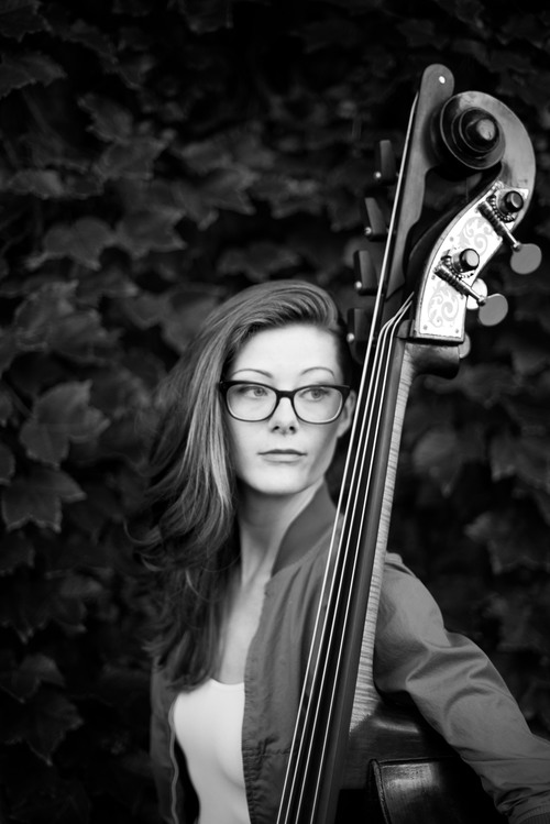
Jordan Morton is a bassist and singer, she regularly performs using both instruments combined. This provides an opportunity to explore how the liveconvolver can work when both the IR and the live input are generated by the same musician. We did a session at UCSD on February 22nd. Here are some reflections and audio excerpts from that session.

General reflections

As compared with playing with live processing, Jordan felt it was more “up to her” to make sensible use of the convolution instrument. With live processing being controlled by another musician, there is also a creative input from another source. In general, electronic additions to the instrument can sometimes add unexpected but desirable aspects to the performance. With live convolution where she is providing both signals, there is a triple (or quadruple) challenge: She needs to decide what to play on the bass, what to sing, explore how those two signals work together when convolved, and finally make it all work as a combined musical statement. It appears this is all manageable, but she’s not getting much help from the outside. In some ways, working with convolution could be compared to looping and overdubs, except the convolution is not static. One can overlay phrases and segments by recording them as IR’s, while shaping their spectral and temporal contour with the triggering sound (the one being convolved with the IR).
Jordan felt it easier to play bass through the vocal IR than the other way around . She tend to lead with the bass when playing acoustic on bass + vocals. The vocals are more an additional timbre added to complete harmonies etc with the bass providing the ground. Maybe the instrument playing through the IR has the opportunity of more actively shaping the musical outcome, while the IR record source is more a “provider” of an environment for the other to actively explore?
In some ways it can seem easier to manage the roles roles (of IR provider and convolution source) as one person than splitting the incentive among two performers. The roles becomes more separated when they are split between different performers than when one person has both roles and then switches between them. When having both roles, it can be easier to explore the nuances of each role. Possible to test out musical incentives by doing this here and then this there , instead of relying on the other person to immediately understand (for example to *keep* the IR, or to *replace* it *now* ).

Technical issues

We explored transient triggered IR recording, but had a significant acoustic bleed from bass into the vocal microphone, which made clean transient trigging a bit difficult. A reliable transient triggered recording would be very convenient, as it would allow the performer to “just play”. We tried using manual triggering, controlled by Oeyvind. This works reliably but involves some guesswork as to what is intended to be recorded. As mentioned earlier (e.g. in the first Olso session ), we could wish for a foot pedal trigger or other controller directly operated by the performer. Hey it’s easy to do, let’s just add one for next time.
We also explored continuous IR updates based on a metronome trigger. This allows periodic IR updates, in a seemingly streaming fashion. Jordan asked for an indication of the metronomic tempo for the updates, which is perfectly reasonable and would be a good idea to do (although had not been implemented yet). One distinct difference noted when using periodic IR updates is that the IR is always replaced. Thus, it is not possible to “linger” on an IR and explore the character of some interesting part of it. One could simulate such exploration by continuously re-recording similar sounds, but it might be more fruitful to have the ability to “hold” the IR, preventing updates while exploring one particular IR. This hold trigger could reasonably also be placed on a footswitch or other accessible control for the performer.

Audio excerpts


Take 1: Vocal IR, recording triggered by transient detection.


Take 2: Vocal IR, manually triggered recording


Take 3: Vocal IR, periodic automatic trigger of IR recording.


Take 4: Vocal IR, periodic automatic trigger of IR recording (same setup as for take 3)


Take 5: Bass IR, transient triggered recording. Transient triggering worked much cleaner on the bass since there was less signal bleed from voice to bass than vice versa.

Crossadaptive session NTNU 12. December 2016

Participants:

Trond Engum (processing musician)

Tone Åse (vocals)

Carl Haakon Waadeland (drums and percussion)

Andreas Bergsland (video)

Thomas Henriksen (sound technician)

Video digest from session:

Session objective and focus:

The main focus in this session was to explore other analysing methods than used in earlier sessions (focus on rhythmic consonance for the drums, and spectral crest on the vocals). These analysing methods were chosen to get a wider understanding of their technical functionality, but also their possible use in musical interplay. In addition to this there was an intention to include the sample/hold function for the MIDIator plug-in. The session was also set up with a large screen in the live room to monitor the processing instrument to all participants at all times. The idea was to democratize the processing musician role during the session to open up for discussion and tuning of the system as a collective process based on a mutual understanding. This would hopefully communicate a better understanding of the functionality in the system, and how the musicians individually can navigate within it through their musical input. At the same time this also opens up for a closer dialog around choice of effects and parameter mapping during the process.

Earlier experiences and process

Following up on experiences documented through earlier sessions and previous blog posts, the session was prepared to avoid the most obvious shortcomings. First of all, separation between instruments to avoid bleeding through microphones was arranged by placing vocals and drums in separate rooms. Bleeding between microphones was earlier affecting both the analysed signals and effects. The system was prepared to be as flexible as possible beforehand containing several effects to map to, flexibility in this context meaning the possibility to do fast changes and tuning the system depending on the thoughts from the musicians. Since the group of musicians remained unchanged during the session this flexibility was also seen as a necessity to go into details and more subtle changes both in the MIDIator and the effects in play to reach common aesthetical intentions.

Due to technical problems in the studio (not connected with the cross adaptive set up or software) the session was delayed for several hours resulting in shorter time than originally planned. We therefore made a choice to concentrate only on rhythmic consonance (referred to as rhythmical regularity in the video) as analysing method for both drums and vocals. The method we used to familiarize with this analysing tool was that we started with drums trying out different playing techniques with both regular and irregular strokes while monitoring the visual feedback from the analyser plug-in without any effect. Regular strokes in this case resulting in high stable value, irregular strokes resulting in low value.

picture1

Figure 1. Consonance (regularity) visualized in the upper graph.

What became evident was that when the input stopped, the analyser stayed at the last measured value, and in that way could act as a sort of sample/hold function on the last value and in that sense stabilise a setting in an effect until an input was introduced again. Another aspect was that the analysing method worked well for regularity in rhythm, but had more unpredictable behaviour when introducing irregularity.

After learning the analyser behaviour this was further mapped to a delay plugging as an adaptive effect on the drums. The parameter controlled the time range of 14 delays resulting in larger delay time range the more regularity, and vice versa.

After fine-tuning the delay range we agreed that the connection between the analyser, MIDIator and choice of effect worked musically in the same direction. (This was changed later in the session when trying out cross-adaptive processing).

The same procedure was followed when trying vocals, but then concentrating the visual monitoring mostly on the last stage of the chain, the delay effect. This was experienced as more intuitive when all settings were mapped since the musician then could interact visually with the input during performance.

Cross-adaptive processing.

When starting the cross-adaptive recording everyone had followed the process, and tried out the chosen analysing method on own instruments. Even though the focus was mainly on the technical aspects the process had already given the musicians the possibility to rehearse and get familiar with the system.

The system we ended up with was set up in the following way:

Both drums and vocals was analysed by rhythmical consonance (regularity). The drums controlled the send volume to a convolution reverb and a pitch shifter on the vocals. The more regular drums the less of the effects, the less regular drums the more of the effects.

The vocals controlled the time range in the echo plugin on the drums. The more regular pulses from the vocal the less echo time range on the drums, the less regular pulses from the vocals the larger echo time range on the drums.

Sound example (improvisation with cross adaptive setup):

Adding new array operations to Csound II: the Mel-frequency filterbank

As I have discussed before in my previous post , as part of this project we have been selecting a number of useful operations to implement in Csound, as part of its array opcode collection. We have looked at the components necessary for the implementation of the Mel-frequency cepstrum coefficient (MFCC) analysis and in this post I will discuss the Mel-frequency filterbank as the final missing piece.

The word filterbank might be a little misleading in this context, as we will not necessarily implement a complete filter. We will design a set of weighting curves that will be applied to the power spectrum. From each one of this we will obtain an average value, which will be the output of the MFB at a given centre frequency. So from this perspective, the complete filter is actually made up of the power spectrum analysis and the MFB proper.

So what we need to do is the following:

  1. Find L evenly-space centre frequencies in the Mel scale (within a minimum and maximum range).
  2. Construct L overlapping triangle-shape curves, centred at each Mel-scale frequency.
  3. Apply each one of these curves to the power spectrum and averaging the result. These will be the outputs of the filterbank.

The power spectrum input comes as sequence of equally-spaced bins. So, to achieve the first step, we need to convert to/from the Mel scale, and also to be able to establish which bins will be equivalent to the centre frequencies of each triangular curve. We will show how this is done using the Python language as an example.

The following function converts from a frequency in Hz to a Mel-scale frequency.

import pylab as pl
def f2mel(f):
  return 1125.*pl.log(1.+f/700.)

mel

With this function, we can convert our start and end Mel values and linearly space the L filter centre frequencies. From these L Mel values, we can get the power spectrum bins using

def mel2bin(m,N,sr):
  f = 700.*(pl.exp(m/1125.) - 1.)
  return  int(f/(sr/(2*N)))

where m is the Mel frequency, N is the DFT size used and sr is the sampling rate. A list of bin numbers can be created, associating each L Mel centre frequency with a bin number

Step 2 is effectively based on creating ramps that will connect each bin in the list above. The following figure demonstrates the idea for L=10, and N=4096 (2048 bins)

mfb
Each triangle starts at a Mel frequency in the list, rises to the next, and decays to the following one (frequencies are quantised to bin centres). To obtain the output for each filter we weigh the bin values (spectral powers) by these curves and then output the average value for each band.

The Python code for the MFB operation is shown below:

def MFB(input,L,min,max,sr):
  """
  From a power spectrum in input, creates an array 
  consisting of L values containing
  its MFB, from a min to a max frequency sampled 
  at sr Hz.
  """
  N = len(input)
  start = f2mel(min)
  end = f2mel(max)
  incr = (end-start)/(L+1)
  bins = pl.zeros(L+2)
  for i in range(0,L+2):
    bins[i] = mel2bin(start,N-1,sr)
    start += incr
  output = pl.zeros(L)
  i = 0
  for i in range(0,L):
    sum = 0.0
    start = bins[i]
    mid = bins[i+1]
    end = bins[i+2]
    incr =  1.0/(mid - start)
    decr =  1.0/(end - mid)
    g = 0.0
    for bin in input[start:mid]:
      sum += bin*g
      g += incr
    g = 1.0
    for bin in input[mid:end]:
      sum += bin*g
      g -= decr
    output[i] = sum/(end - start) 
  return output

We can demonstrate the use of the MFB  by plotting the output of a N=4096, L=128 full-spectrum magnitude analysis of a flute tone.
mfb2

We can see how the MFB identifies clearly the signal harmonics. Of course, the original application we had in mind (MFCCs) is significantly different from this one, but this example shows what kinds of outputs we should expect from the MFB.

Evolving Neural Networks for Cross-adaptive Audio Effects

I’m Iver Jordal and this is my first blog post here. I have studied music technology for approximately two years and computer science for almost five years. During the last 6 months I’ve been working on a specialization project which combines cross-adaptive audio effects and artificial intelligence methods. Øyvind Brandtsegg and Gunnar Tufte were my supervisors.

A significant part of the project has been about developing software that automatically finds interesting mappings (neural networks) from audio features to effect parameters. One thing that the software is capable of is making one sound similar to another sound by means of cross-adaptive audio effects. For example, it can process white noise so it sounds like a drum loop.

Drum loop (target sound):

White noise (input sound to be processed):

Since the software uses algorithms that are based on random processes to achieve its goal, the output varies from run to run. Here are three different output sounds:

These three sounds are basically white noise that have been processed by distortion and low-pass filter. The effect parameters were controlled dynamically in a way that made the output sound like the drum loop (target sound).

This software that I developed is open source, and can be obtained here:

https://github.com/iver56/cross-adaptive-audio

It includes an interactive tool that visualizes output data and lets you listen to the resulting sounds. It looks like this:

visualization-screenshot
For more details about the project and the inner workings of the software, check out the project report:

Evolving Artificial Neural Networks for Cross-adaptive Audio (PDF, 2.5 MB)

Abstract:

Cross-adaptive audio effects have many applications within music technology, including for automatic mixing and live music. The common methods of signal analysis capture the acoustical and mathematical features of the signal well, but struggle to capture the musical meaning. Together with the vast number of possible signal interactions, this makes manual exploration of signal mappings difficult and tedious. This project investigates Artificial Intelligence (AI) methods for finding useful signal interactions in cross-adaptive audio effects. A system for doing signal interaction experiments and evaluating their results has been implemented. Since the system produces lots of output data in various forms, a significant part of the project has been about developing an interactive visualization tool which makes it easier to evaluate results and understand what the system is doing. The overall goal of the system is to make one sound similar to another by applying audio effects. The parameters of the audio effects are controlled dynamically by the features of the other sound. The features are mapped to parameters by using evolved neural networks. NeuroEvolution of Augmenting Topologies (NEAT) is used for evolving neural networks that have the desired behavior. Several ways to measure fitness of a neural network have been developed and tested. Experiments show that a hybrid approach that combines local euclidean distance and Nondominated Sorting Genetic Algorithm II (NSGA-II) works well. In experiments with many features for neural input, Feature Selective NeuroEvolution of Augmenting Topologies (FS-NEAT) yields better results than NEAT.

The Analyzer and MIDIator plugins

… so with all these DAW examples “where are the plugins” you might ask. Well, the most up-to-date versions will always be available in the code repo at github . BUT, I’ve also uploaded precompiled versions of the plugins for Windows and OSX . To install them you just unzip and put them somewhere in your VST plugin search path (typically /Program Files/Vstplugins on windows and /Library/Audio/Plugins/VST on OSX). You also need to install Cabbage to make them work. You can find the latest Cabbage versions here .