Exploring radically new modes of musical interaction in live performance
Category: Sessions
Session with Kim Henry Ortveit
February 22, 2018
-
Kim Henry is currently a master student at NTNU music technology, and as part of his master project he has designed a new hybrid instrument. The instrument allows close interactions between what is played on a keyboard (or rather a ...
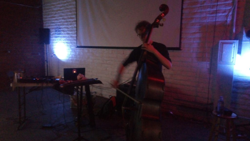
Session with Michael Duch
February 22, 2018
-
February 12th, we did a session with Michael Duch on double bass, exploring auto-adaptive use of our techniques. We were interested in seeing how the crossadaptive techniques could be used for personal timbral expansion for a single player. This is ...
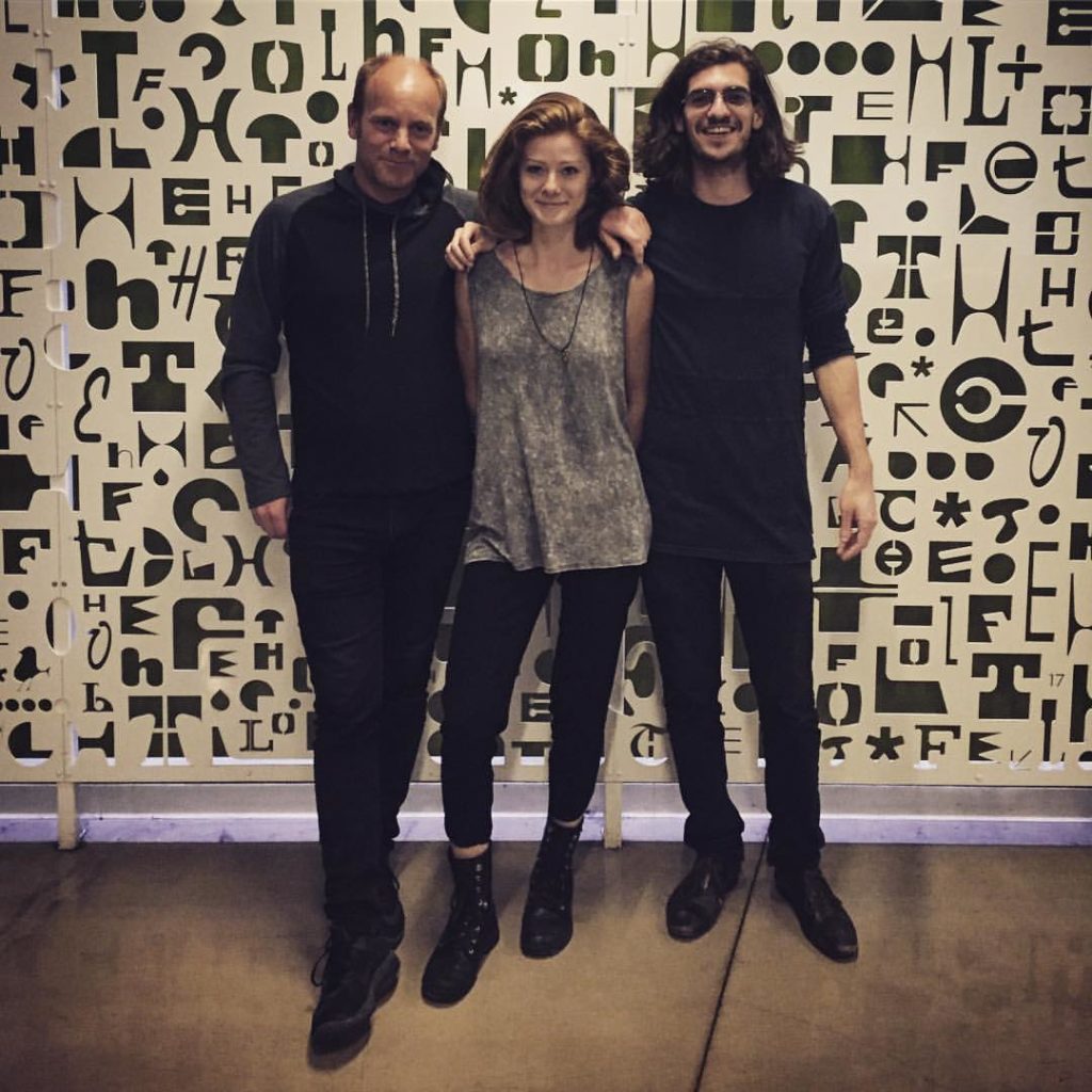
Session with David Moss in Berlin
February 2, 2018
-
Thursday February 1st, we had an enjoyable session at the Universität der Kunste in Berlin. This was at the Grunewaldstraße campus and generously hosted by professor Alberto De Campo. This was a nice opportunity to follow up on earlier collaboration ...
Session with 4 singers, Trondheim, August 2017
October 9, 2017
-
Location: NTNU, Studio Olavshallen. Date: August 28 2017 Participants: Sissel Vera Pettersen, vocals Ingrid Lode, vocals Heidi Skjerve, vocals Tone Åse, vocals Øyvind Brandtsegg, processing Andreas Bergsland, observer and video documentation Thomas Henriksen, sound engineer Rune Hoemsnes, sound engineer We ...
Session in UCSD Studio A
September 8, 2017
-
This session was done May 11th in Studio A at UCSD. I wanted to record some of the performer constellations I had worked with in San Diego during Fall 2016 / Spring 2017. Even though I had worked with all ...
Session with Jordan Morton and Miller Puckette, April 2017
June 9, 2017
-
This session was conducted as part of preparations to the larger session in UCSD Studio A, and we worked on calibration of the analysis methods to Jordans double bass and vocals. Some of the calibration and accomodation of signals also includes ...
Liveconvolver experiences, San Diego
June 7, 2017
-
The liveconvolver has been used in several concerts and sessions in San Diego this spring. I played three concerts with the group Phantom Station (The Loft, Jan 30th, Feb 27th and Mar 27th), where the first involved the liveconvolver. Then ...
Live convolution session in Oslo, March 2017
June 7, 2017
-
Participants: Bjørnar Habbestad (flute), Bernt Isak Wærstad (guitar), Gyrid Nordal Kaldestad (voice) Mats Claesson (documentation and observation). The focus for this session was to work with the new live convolver in Ableton Live Setup - getting to know the Convolver We ...
Second session at Norwegian Academy of Music (Oslo) – January 13. and 19., 2017
June 7, 2017
-
Participants: Bjørnar Habbestad (flute), Bernt Isak Wærstad (guitar), Gyrid Nordal Kaldestad (voice) The focus for this session was to play with, fine tune and work further on the mappings we sat up during the last session at NMH in November. Due ...
Cross adaptive session with 1st year jazz students, NTNU, March 7-8
April 6, 2017
-
This is a description of a session with first year jazz students at NTNU recorded March 7 and 8. The session was organized as part of the ensemble teaching that is given to jazz students at NTNU, and was meant to take care ...
Live convolution with Kjell Nordeson
March 23, 2017
-
Session at UCSD March 14. Kjell Nordeson: Drums Øyvind Brandtsegg: Vocals, Convolver. Contact mikes In this session, we explore the use of convolution with contact mikes on the drums to reduce feedback and cross-bleed. There is still some bleed from ...
Session with classical percussion students at NTNU, February 20, 2017
March 10, 2017
-
Introduction: This session was a first attempt in trying out cross-adaptive processing with pre-composed material. Two percussionists, Even Hembre and Arne Kristian Sundby, students at the classical section, were invited to perform a composition written for two tambourines. The musicians ...
Convolution experiments with Jordan Morton
March 1, 2017
-
Jordan Morton is a bassist and singer, she regularly performs using both instruments combined. This provides an opportunity to explore how the liveconvolver can work when both the IR and the live input are generated by the same musician. We did a ...
Docmarker tool
February 16, 2017
-
Docmarker During our studio sessions and other practical research work sessions, we noted that we needed a tool to annotate documentation streams. The stream could be an audio file, a video or some line of timed events. Audio editors and ...
Session UCSD 14. Februar 2017
February 15, 2017
-
Session objective The session objective was to explore the live convolver, how it can affect our playing together and how it can be used. New convolver functionality for this session is the ability to trigger IR update via transient detection, ...
Crossadaptive session NTNU 12. December 2016
December 16, 2016
-
Participants: Trond Engum (processing musician) Tone Åse (vocals) Carl Haakon Waadeland (drums and percussion) Andreas Bergsland (video) Thomas Henriksen (sound technician) Video digest from session: https://www.youtube.com/watch?v=ktprXKVdqF4&feature=youtu.be Session objective and focus: The main focus in this session was to explore other ...
Oslo, First Session, October 18, 2016
December 12, 2016
-
First Oslo Session. Documentation of process 18.11.2016 Participants Gyrid Kaldestad, vocal Bernt Isak Wærstad, guitar Bjørnar Habbestad, flute Observer and Video Mats Claesson The Session took place in one of the sound studios at the Norwegian Academy of Music, Oslo ...
Multi-camera recording and broadcasting
November 21, 2016
-
Audio and video documentaion is often an important component of projects that analyse or evaluate musical performance and/or interaction. This is also the case in the Cross Adaptive project where every session was to be recorded in video and multi-track ...
Session 19. October 2016
October 31, 2016
-
Location: Kjelleren, Olavskvartalet, NTNU, Trondheim Participants: Maja S. K. Ratkje, Siv Øyunn Kjenstad, Øyvind Brandtsegg, Trond Engum, Andreas Bergsland, Solveig Bøe, Sigurd Saue, Thomas Henriksen Session objective and focus Although the trio BRAG RUG has experimented with crossadaptive techniques in rehearsals and ...
Session 20. – 21. September
September 30, 2016
-
Location: Studio Olavskvartalet, NTNU, Trondheim Participants: Trond Engum, Andreas Bergsland, Tone Åse, Thomas Henriksen, Oddbjørn Sponås, Hogne Kleiberg, Martin Miguel Almagro, Oddbjørn Sponås, Simen Bjørkhaug, Ola Djupvik, Sondre Ferstad, Björn Petersson, Emilie Wilhelmine Smestad, David Anderson, Ragnhild Fangel Session objective and focus: This post is a description of a session with 3rd year Jazz students at NTNU. It was the first session following the intended procedure ...
Mixing with Gary
June 16, 2016
-
During our week in London we had some sessions with Gary Bromham, first at the Academy of Contemporary Music in Guildford on the June 7th , then at QMUL later in the week. We wanted to experiment with cross-adpative techniques ...
Mixing example, simplified interaction demo
May 24, 2016
-
When working further with some of the examples produced in an earlier session , I wanted to see if I could demonstrate the influence of one instrument's influence of the the other instruments sound more clearly. Here' I've made an example where the ...
Introductory session NTNU, Trond/Øyvind
May 13, 2016
-
Date: 3 May 2016 Location: NTNU Mustek Participants: Trond Engum, Øyvind Brandtsegg Session objective and focus: Test ourselves as musicians in cross adaptive setting. MEaning, test how we react to being in the role of the processed Test out different mappings, ...
Introductory session, NTNU, Bernt/Øyvind
May 13, 2016
-
Date: 26 April 2016 Location: NTNU Mustek Participants: Bernt Isak Wærstad, Øyvind Brandtsegg Session objective and focus: Test ourselves as musicians in cross adaptive setting. We have usually been the processing musicians, now we should test ourselves as the victims ...
Westerdal session April 2016
May 13, 2016
-
Session at Westerdal ACT, OSLO Participants: Ylva Øyen Brandtsegg, Øyvind Brandtsegg Objective: Studio use of cross_shimmer effect Takes Take 1: Cross_shimmer: Vocals as spectral input, Drumset as exciter Take2: As above, another take on the same musical goal Comments: * Feedback not ...
Tape to zero 2016
May 13, 2016
-
Concert : Tape to zero festival, April 21 2016, Victoria Jazz, Nasjonal jazzscene Oslo Participants: Maja S.K. Ratkje, Siv Øyunn Kjenbstad, Øyvind Brandtsegg The objective, in the context of this research project, was live use of the "cross_shimmer" effect, testing musical applications ...
Jazz ensemble, spring 2016
May 13, 2016
-
Experimental session in the context of ensemble teaching at the jazz dept at NTNU, April 2016. The objective was to test some simple interaction modes, starting with cross adaptive amplitude control. How will the musicians react to this kind of interaction? ...
This session was conducted as part of preparations to the larger session in UCSD Studio A, and we worked on calibration of the analysis methods to Jordans double bass and vocals. Some of the calibration and accomodation of signals also includes the fun creative work of figuring out which effects and which effect parameters to map the analyses to. The session resulted in some new discoveries in this respect, for example using the spectral flux of the bass to control vocal reverb size, and using transient density to control very low range delay time modulations. Among the issues we discussed were aspects of
timbral polyphony,
i.e. how many simultaneous modulations can we percieve and follow?
The liveconvolver has been used in several concerts and sessions in San Diego this spring. I played three concerts with the group
Phantom Station
(
The Loft
, Jan 30th, Feb 27th and Mar 27th), where the first involved the liveconvolver. Then one concert with the band
Creatures
(
The Loft
, April 11th), where the live convolver was used with contact mikes on the drums, and live sampling IR from the vocals. I also played a duo concert with
Kjell Nordeson
at
Bread and Salt
April 13th, where the liveconvolver was used with contact mikes on the drums, live sampling IR from my own vocals. Then a duo concert with
Kyle Motl
at
Coaxial
in L.A (April 21st), where a combination of crossadaptive modulation and live convolver was used. For the duo with Kyle, I switched between using bass as the IR and vocals as the IR, letting the other instrument play through the convolver. A number of studio sessions was also conducted, with Kjell Nordeson, Kyle Motl, Jordan Morton, Miller Puckette, Mark Dresser, and Steven Leffue. A separate report on the studio sesssion in
UCSD Studio A
will be published later.
“Phantom Station”, The Loft, SD
This group is based on Butch Morris’
conduction
language for improvisation, and the performance typically requires a specific action (specific although it is free and open) to happen on cue from the conductor. I was invited into this ensemble and encouraged to use whatever part of my instrumentarium that I might see fit. Since I had just finished the liveconvoolver plugin, I wanted to try that out. I also figured my live processing techniques would fit easily, in case the liveconvolver did not work so well. Both the live processing and the live convolution instruments was in practice less than optimal for this kind of ensemble playing. Even though the instrumental response can be fast (low latency), the way I normally use these instruments
is not
for making a musical statements quickly for one second and then suddenly stop again. This leads me to reflect on a quality measure I haven’t really thought of before. For lack of a better word, let’s call it
reactive inertia
: the possibility to completely change direction on the basis of some external and unexpected signal. This is something else than the
audio latency
(of the audio processing) and also something else than the
user interface latency
(like for example, the time it takes the performer to figure out which button to turn to achieve a desired effect). I think it has to do with the sound production process, for example how some effects take time to build up before they are heard as a distinct musical statement, and also the inertia due to interaction between humans and also the signal chain of sound production pre effects (say if you live sample or live process someone, need to get a sample, or need to get some exciter signal). For live interaction instruments, the
reactive inertia
is then goverened by the time it takes two performers to react to the external stimuli, and their combined efforts to be turned into sound by the technology involved. Much like what an old man once told me at Ocean Beach:
“There’s two things that needs to be ready for you to catch a wave
– You, …and the wave”.
We can of course prepare for sudden shifts in the music, and construct instruments that will be able to produce sudden shifts and fast reactions. Still, the reaction to a completely unexpected or unfamiliar stimuli will be slower than optimal. An acoustic instrument has less of these limitations. For this reason, I switched to using the Marimba Lumina for the remaning two concerts with Phantom Station, to be able to shape immediate short musical statements with more ease.
Phantom Station
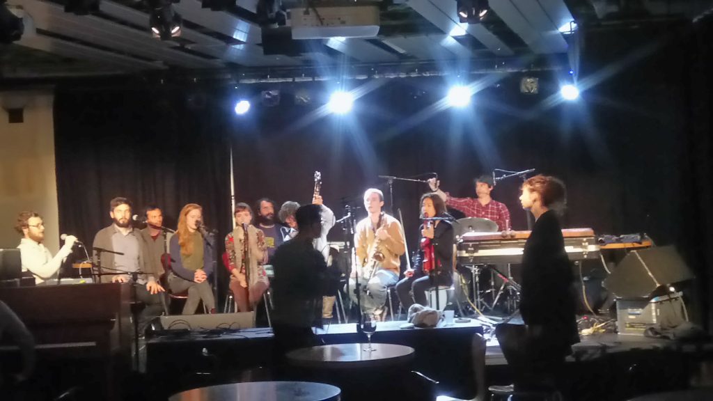
“Creatures”, The Loft, SD
Creatures
is the duo of Jordan Morton (double bass, vocals) and Kai Basanta (drums). I had the pleasure of sitting in with them, making it a trio for this concert at
The Loft
.
Creatures
have some composed material in the form of songs, and combine this with long improvised stretches. For this concert I got to explore the liveconvolver quite a bit, in addition to the regular live processing and Marimba Lumina. The convolver was used with input from piezo pickups on the drums, convolving with IR live recorded from vocals. Piezo pickups can be very “impulse-like”, especially when used on percussive instruments. The pickups’ response have a generous amount of high frequencies, and a very high dynamic range. Due to the peaky impulse-like nature of the signal, it drives the convolution almost like a sample playback trigger, creating delay patterns on the input sound. Still the convolver output can become sustained and dense, when there is high activity on the triggering input. In the live mix, the result sounds somewhat similar to infinite reverb or “freeze” effects (using a trigger to capture a timbral snippet and holding that sound as long as the trigger is enabled). Here, the capture would be the IR recording, and the trigger to create and sustain the output is the activity on the piezo pickup. The
causality
and
performer interface
is very different than that of a freeze effect, but listening to it from the outside, the result is similar. These expressive limitations can be circumvented by changing the miking technique, and working in a more directed way as to what sounds goes into the convolver. Due to the relatively few control parameters, the main thing deciding how the convolver sounds is the input signals. The term
causality
in this context was used by Miller Puckette when talking about the relationship between performative actions and instrumental reactions.
Creatures + Brandtsegg
Creatures at The Loft. A liveconvolver example can be found at 29:00 to 34:00 with Vocal IR, and briefly around 35:30 with IR from double bass.
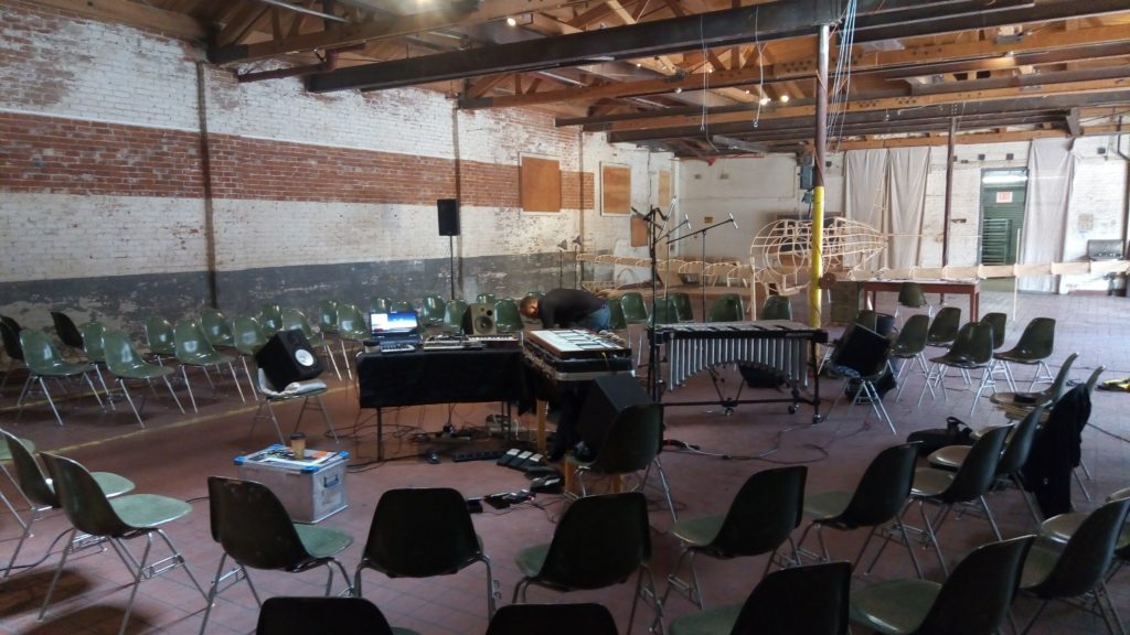
“Nordeson/Brandtsegg duo”, Bread & Salt, SD
Duo configuration, where Kjell plays drums/perc and vibraphone, and I did live convolution, live processing and Marimba Lumina. My techniques was much like what I used with
Creatures
. The live convolver setup was also similar, with IR being live sampled from my vocals and the convolver being triggered by piezo pickups on Kjell’s drums. I had the opportunity to work over a longer period of time preparing for this concert together with Kjell. Because if this, we managed to develop a somewhat more nuanced utilization of the convolver techniques. Still, in the live performance situation on a PA, the technical situation made it a bit more difficult to utilize the fine grained control over the process and I felt the sounding result was similar in function to what I did together with Creatures. It works well like this, but there is potential for getting a lot more variation out of this technique.
Nordeson and Brandtsegg setup at Bread and Salt
We used a quadrophonic PA setup for this concert. Due to an error with the front-of-house patching, only 2 of the 4 lines from my electronics was recorded. Due to this fact, the mix is somewhat off balance. The recording also lacks first part of the concert, starting some 25 minutes into it.
“The Gringo and the Desert”, Coaxial, LA
In this duo Kyle Motl plays double bass and I do vocals, live convolution, live processing, and also crossadaptive processing. I did not use the Marimba Lumina in this setting, so some more focus was allowed for the processing. In terms of crossadaptive processing, the utilization of the techniques is a bit more developed in this configuration. We’ve had the opportunity to work over several months, with dedicated rehearsal sessions focusing on separate aspects of the techniques we wanted to explore. As it happpened during the concert, we played one long set and the different techniques was enabled as needed. Parameters that was manually controlled in parts of the set, was then delegated to crossadaptive modulations in other parts of the set. The live convolver was used freely as one out of several active live processing modules/voices. The liveconvolver with vocal IR can be heard for example from 16:25 to 20:10. Here, the IR is recorded from vocals, and the process acts as a vocal “shade” or “pad”, creating long sustained sheets of vocal sound triggeered by the double bass. Then, liveconvolver with bass IR from 20:10 to 23:15, where we switch on to full crossadaptive modulation until the end of the set. We used a complex mapping designed to respond to a variety of expressive changes. Our attitude/approach as performers was not to intellectually focus on controlling specific dimensions but to allow the adaptive processing to naturally follow whatever happened in the music.
Gringo and the Desert soundcheck at Coaxial, L.A
Gringo and the Desert at Coaxial DTLA, …yes the backgorund noise is the crickets outside.
Session with Steven Leffue (Apr 28th, May 5th)
I did two rehearsal sessions together with Steven Leffue in April, as preparation for the UCSD Studio A session in May. We worked both on crossadaptive modulations and on live convolution. Especially interesting with Steven is
his own use of adaptive and crossadaptive techniques
. He has developed a setup in PD, where he tracks
transient density
and
amplitude envelope
over different time windows, and also uses
standard deviation
of transient density within these windows. The windowing and statistics he use can act somewhat like a feature we have also discussed in our crossadaptive project: a method of making an analysis “in relation to the normal level” for a given feature. Thus, a way to track relative change. Steven’s Master thesis
“Musical Considerations in Interactive Design for Performance”
relates to this and other issues of adaptive live performance. Notable is also his ICMC paper
“AIIS: An Intelligent Improvisational System”
. His music can be heard at
http://www.stevenleffue.com/music.html
, where the adaptive electronics is featured in “A theory of harmony” and “Futures”.
Our first session was mainly devoted to testing and calibrating the analysis methods towards use on the saxophone. In very broad terms, we notice that the different analysis streams now seem to work relatively similar on different instruments. The main diffferences are related to extraction of tone/noise balance, general brightness, timbral “pressedness” (weight of formants), and to some extent in transient detection and pitch tracking. The reason why the analysis methods now appear more robust is partly due to refinements in their implementation, and partly due to (more) experience in using them as modulators. Listening, experimentation, tweaking, and plainly just a lot of spending-time-with-them, have made for a more intuitive understanding of how each analysis dimension relates to an audio signal.
The second session was spent exploring live convolution between Sax and Vocals. Of particular interest here is the comments from Steven regarding the performative roles of IR recording vs playing the convolver. Steven states quite strongly that
the one recording the IR has the most influence over the resulting music
. This impression is consistent when he records the IR (and I sing through it), and when I record the IR and he plays through it. This may be caused by several things, but of special interest is that it is
diametrically opposed
to what many other performers have stated. Both
Kyle
,
Jordan
and
Kjell
in our initial sessions, voiced a
higher performative intimacy
, a
closer connection
to the output when playing through the IR. Maybe Steven is more concerned with the resulting timbre (including processed sound) than the physical control mechanism, as he routinely designs and performs with his own interactive electronics rig. Of course all musician care about the sound, but perhaps there is a difference of approach on just
how to get there
. With the liveconvolver we put the performers in an unfamiliar situation, and the differences in approach might just show different methods of problems solving to gain control over this situation. What I’m trying to investigate is how the liveconvolver technique works performatively, and in this, the performer’s personal and musical traits plays into the situation quite strongly. Again, we can only observe single occurences and try to extract things that might work well. There is no conclusions to be drawn on a general basis as to what works and what does not, and neither can we conclude what is the nature of this situation and this tool. One way of looking at it (I’m still just guessing) is that Steven treats the convolver as *
the environment
* in which music can be made. The changes to the environment determines what can be played and how that will sound, and thus, the one recording the IR controls the environment and subsequently controls the most important factor in determining the music.
In this session, we also experimented a bit with transposed and revesed IR, this being some of the parametric modifications we can make to the IR with our liveconvolver technique. Transposing can be interesting, but also quite difficult to use musically. Transposing in octave intervals can work nicely, as it will act just as much as a timbral colouring without changing pitch class. A fun fact about reversed IR as used by Steven: If he played in the style of Charlie Parker and we reversed the IR, it would sound like Evan Parker. Then, if he played like Evan Parker and we reversed the IR, it would still sound like Evan Parker. One could say this puts Evan Parker at the top of the convolution-evolutionary-saxophone tree….
Steven Leffue
Liveconvolver experiment Sax/Vocals, IR recorded by vocals.
Liveconvolver experiment Sax/Vocals, IR recorded by Sax.
Liveconvolver experiment Sax/Vocals, time reversed IR recorded by Sax.
Session with Miller Puckette, May 8th
The session was intended as “calibration run”, to see how the analysis methods responded to Miller’s guitar. This as a preparation for the upcoming bigger session in UCSD Studio A. The main objective was to determine which analysis features would work best as expressive dimensions, find the appropriate ranges, and start looking at potentially useful mappings. After this, we went on to explore the liveconvolver with vocals and guitar as the input signals. Due to the “calibration run” mode of approach, the session was not videotaped. Our comments and discussion was only dimly picked up by the microphones used for processing. Here’s a transcription of some of Millers initial comments on playing with the convolver:
“It is interesting, that …you can control aspects of it but never really control the thing. The person who’s doing the recording is a little bit less on the hook. Because there’s always more of a delay between when you make something and when you hear it coming out [when recording the IR]. The person who is triggering the result is really much more exposed, because that person is in control of the timing. Even though the other person is of course in control of the sonic material and the interior rhythms that happen.”
Since the liveconvolver has been developed and investigated as part of the research on crossadaptive techniques, I had slipped into the habit of calling it a crossadaptive technique. In discussion with Miller, he pointed out that the liveconvolver is not really *crossadaptive* as such. BUT it involves some of the same performative challenges, namely playing something that is not played solely for the purpose of it’s own musical value. The performers will sometimes need to play something that will affect the sound of the other musician in some way. One of the challenges is how to incorporate that thing into the musical narrative, taking care of how it sounds in itself, and exactly how it will affect the other performer’s sound. Playing with liveconvolver has this performative challenge, as has the regular crossadaptive modulation. One thing the live convolver does not have is the reciprocal/two-way modulation, it is more of a one-way process. The
recent Oslo session on liveconvolution
used two liveconvolvers simultaneously to re-introduce the two-way reciprocal dependency.
Miller Puckette
Liveconvolver experiment Guitar/Vocals, IR recorded by guitar.
Liveconvolver experiment Guitar/Vocals, IR recorded by guitar.
Liveconvolver experiment Guitar/Vocals, IR recorded by guitar.
Liveconvolver experiment Guitar/Vocals, IR recorded by vocals.
Liveconvolver experiment Guitar/Vocals, IR recorded by vocals.
The focus for this session was to play with, fine tune and work further on the mappings we sat up during the last session at NMH in November. Due to practical reasons, we had to split the session into two half days on 13th and 19th of January
13
th
of January 2017
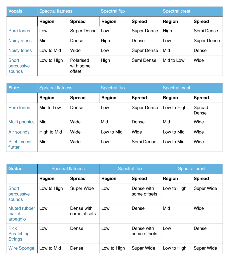
We started by analysing 4 different musical gestures for the guitar, which was skipped due to time constraints during the last session. During this analysis we found the need to specify the spread of the analysis results in addition to the region. This way we could differentiate the analysis results in terms of stability and conclusiveness. We decided to analyse the flute and vocal again to add the new parameters.
19
th
of January 2017
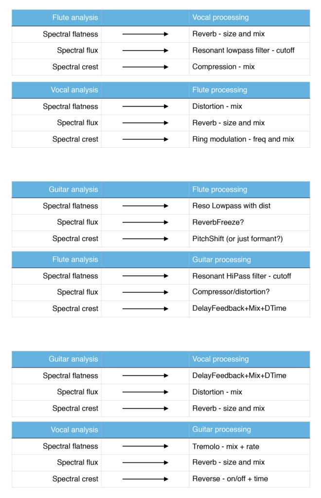
After the analysis was done, we started working on a mapping scheme which involved all 3 instruments, so that we could play in a trio setup. The mappings between flute and vocal where the same as in the November session
The analyser was still run in Reaper, but all routing, effects chain and mapping (MIDIator) was now done in Live. Because of software instability (the old Reaper projects from November wouldn’t open) and change of DAW from Reaper to Live, meant that we had to set up and tune everything from scratch.
Sound examples with comments and immediate reflections
1. Guitar & Vocal
– First duo test, not ideal, forgot to mute analyser.
2. Guitar & Vocal retake
– Listened back on speakers after recording. Nice sounding. Promising.
Reflection: There seems to be some elements missing, in a good way, meaning that there is space left for things to happen in the trio format. There is still need for fine-tuning of the relationship between guitar and vocal. This scenario stems from the mapping being done mainly with the trio format in mind.
3. Vocals & flute
– Listened back on speakers after recording.
Reflections: dynamic soundscape, quite diverse results, some of the same situations as with take 2, the sounds feel complementary to something else. Effect tuning: more subtle ring mod (good!) compared to last session, the filter on vocals is a bit too heavy-handed. Should we flip the vocal filter? This could prevent filtering and reverb taking place simultaneously. Concern: is the guitar/vocal relationship weaker compared to vocal/flute? Another idea comes up – should we look at connecting gates or bypasses in order to create dynamic transitions between dry and processed signals?
4.Flute & Guitar
Reflections: both the flute ring mod and git delay are a bit on the heavy side, not responsive enough. Interesting how the effect transformations affect material choices when improvising.
5.Trio
Comments and reflections after the recording session
It is interesting to be in a situation where you, as you play, are having multi-layered focuses- playing, listening, thinking of how you affect the processing of your fellow musicians and how your sound is affected and trying to make something worth listening to. Of course we are now in an “etyde- mode”, but still striving for the goal, great output!
It seems to be a bug in the analyser tool when it comes to being consistent. Sometimes some parameters fall out. We experienced that it seems to be a good idea to run the analyse a couple of times for each sound to get the most precise result.
This is a description of a session with first year jazz students at NTNU recorded March 7 and 8. The session was organized as part of the ensemble teaching that is given to jazz students at NTNU, and was meant to take care of both the learning outcomes from the normal ensemble teaching, and also aspects related to the cross adaptive project.
Musicians:
Håvard Aufles, Thea Ellingsen Grant, Erlend Vangen Kongstorp, Rino Sivathas, Øyvind Frøberg Mathisen, Jonas Enroth, Phillip Edwards Granly, Malin Dahl Ødegård and Mona Thu Ho Krogstad.
Processing musician:
Trond Engum
Video documentation:
Andreas Bergsland
Sound technician:
Thomas Henriksen
Video digest from the session:
Preparation:
Based on our earlier experiences with bleeding between microphones we located instruments in separate rooms. Since there was quit a big group of different performers it was important that changing set-up took as little time as possible. There was also prepared a system set-up beforehand based on the instruments in use. To gain an understanding of the project from the performer side as early in the process as possible we used the same four step chronology when introducing the performers to the set-up.
Start with individual instruments trying different effects through live processing and decide together with the performers what effects most suitable to add to their instrument.
Introducing the analyser and decide, based on input form the performers, which methods best suited for controlling different effects from their instrument.
Introducing adaptive processing were one performer is controlling the effects on the other, and then repeat vice versa.
Introducing cross-adaptive processing were all previous choices and mappings are opened up for both performers.
Session report:
Day 1. Tuesday 7
th
March
Trumpet and drums
Sound example 1:
(Step 1) Trumpet live processed with two different effects, convolution (impulse response from water) and overdrive.
The performer was satisfied with the chosen effects, also because the two were quite different in sound quality. The overdrive was experienced as nice, but he would not like to have it present all the time. We decided to save these effects for later use on trumpet, and be aware of dynamic control on the overdrive.
Sound example 2:
(Step 1) Drums live processed with dynamically changing delay and a pitch shift 2 octaves down. The performer found the chosen effects interesting, and the mapping was saved for later use.
Sound example 3:
(Step 1) Before entering the analyser and adaptive processing we wanted to try playing together with the effects we had chosen to see if they blended well together. The trumpet player had some problems with hearing the drums during the performance, felt as they were a bit in the background. We found out that the direct sound of the drums was a bit low in the mix, and this was adjusted. We discussed that it is possible to make the direct sound of both instruments louder or softer depending what the performer wants to achieve.
Sound example 4.
(Step 2/3) For this example we entered into the analyser using transient density on drums. This was tried out by showing the analyser at the same time as doing an accelerando on drums. This was then set up as an adaptive control from drums on the trumpet. For control, the trumpet player had a suggestion that the more transient density the less convolution effect was added to the trumpet (less send to a convolution effect with a recording of water). The reason for this was that it could make more sense to have more water on slow ambient parts than on the faster hectic parts. At the same time he suggested that the opposite should happen when adding overdrive to the trumpet by transient density meaning that the more transient density the more overdrive on the trumpet. During the first take a reverb was added to the overdrive in order to blend the sound more into the production. It felt like the dynamical control over the effects was a bit difficult because the water disappeared to easily, and the overdrive was introduced to easily. We agreed to fine-tune the dynamical control before doing the actual test that is present as sound example 4.
Sound example 5:
For this example we changed roles and enabled the trumpet to control the drums (adaptive processing). We followed a suggestion from the trumpet player and used pitch as an analyses parameter. We decided to use this to control the delay effect on the drums. Low notes produced long gaps between delays, whereas high notes produced small gap between delays. This was maybe not the best solution for getting good dynamical control, but we decide to keep this anyway.
Sound example 6:
Cross adaptive performance using the effects and control mappings introduced in example 4 and 5. This was a nice experience for the musicians. Even though it still felt a bit difficult to control it was experienced as musical meaningful. Drummer: “Nice to play a steady grove, and listen to how the trumpet changed the sound of my instrument”.
Vocals and piano
Sound example 7:
We had now changed the instrumentation over to vocals and piano, and we started with a performance doing live processing on both instruments. The vocals were processed using two different effects using a delay, and convolution through a recording of small metal parts. The piano was processed using an overdrive and convolution through water.
Sound example 8:
Cross adaptive performance where the piano was analysed by rhythmical consonance controlling the delay effect on vocals. The vocal was analysed by transient density controlling the convolution effect on the piano. Both musicians found this difficult, but musically meaningful. Sometimes the control aspect was experienced as counterintuitive to the musical intention. Pianist: It felt like there was a 3rd musician present.
Saxophone self-adaptive processing
Sound example 9:
We started with a performance doing live processing to familiarize the performer with the effects. The performer found the augmentation of extended techniques as clicks and pops interesting since this magnified “small” sounds.
Sound example 10:
Self-adaptive processing performances where the saxophone was analysed by transient density and then used to control two different convolution effects (recording of metal parts and recording of a cymbal). The first one resulting in a delay effect the second as a reverb. The higher transient density in the analyses the more delay and less reverb and vice versa. The performer experienced the quality of the effects quit similar so we removed the delay effect.
Sound example 11:
Self-adaptive processing performances using the same set-up but changing the delay effect to overdrive. The use of overdrive on saxophone did not bring anything new to the table the way it was set up since the acoustic sound of the instrument could sound similar to the effect when putting in strong energy.
Day 2. Wednesday 8
th
March
Saxophone and piano
Sound example 12:
Performance with saxophone and live processing, familiarizing the performer with the different effects and then choose which of the effects to bring further into the session. Performer found this interesting and wanted to continue with reverb ideas.
Sound example 13:
Performance with piano and live processing. The performer especially liked the last part with the delays – Saxophonist: “It was like listening to the sound under water (convolution with water) sometimes, and sometimes like listening to an old radio (overdrive)”. Piano wanted to keep the effects that were introduced.
Sound example 14:
Adaptive processing, controlling delay on saxophone from the piano by using analyses of the transient density. The higher transient density, the larger gap between delays on the saxophone. The saxophone player found it difficult to interact since the piano had a clean sound during performance. The piano on the other hand felt in control over the effect that was added.
Sound example 15:
Adaptive processing using saxophone to control piano. We analyzed the rhythmical consonance on saxophone. The higher degree of consonance, the more convolution effect (water) was added to piano and vice versa. Saxophone didn’t feel in control during performance, and guessed it was due to not holding a steady rhythm over a longer period. The direct sound of the piano was also a bit loud in the mix making the added effect a bit low in the mix. Piano felt that saxophone was in control, but agreed to the point that the analyses was not able to read to the limit because of the lack of a steady rhythm over a longer time period.
Sound example 16:
Crossadptive performance using the same set-up as in example 14 and 15. Both performers felt in control, and started to explore more of the possibilities. Interesting point when the saxophone stops to play since the rhythmical consonance analyses will make a drop as soon as it starts to read again. This could result in strong musical statements.
Sound example 17:
Crossadaptive performance keeping the same setting but adding rms analyses on the saxophone to control a delay on the piano (the higher rms the less delay and vice versa).
Vocals and electric guitar
Sound example 18:
Performance with vocals and live processing. Vocalist: “It is fun, but something you need to get use to, needs a lot of time”.
Sound example 19:
Performance with Guitar and live processing. Guitarist: “Adapted to the effects, my direct sound probably sounds terrible, feel that I`m loosing my touch, but feels complementary and a nice experience”.
Sound example 20:
Performance with adaptive processing. Analyzing the guitar using rms and transient density. The higher transient density the more delay added to the vocal, and higher rms the less reverb added to the vocal. Guitar: I feel like a remote controller and it is hard to focus on what I play sometimes. Vocalist: “Feels like a two dimensional way of playing”.
Sound example 21:
Performance with adaptive processing. Controlling the guitar by vocals. Analyzing the rhythmical consonance on the vocal to control the time gap between delays inserted on the guitar. Higher rhythmical consonance results in larger gaps and vice versa. The transient density on vocal controls the amount of pitch shift added to the guitar. The higher transient density the less volume is sent to the pitch shift.
Sound example 22:
Performance with cross adaptive processing using the same settings as in sound example 20 and 21.
Vocalist: “It is another way of making music, I think”. Guitarist: “I feel control and I feel my impact, but musical intention really doesn’t fit with what is happening – which is an interesting parameter. Changing so much with doing so little is cool”.
Observation and reflections
The sessions has now come to a point were there is less time used on setting up and figuring out how the functionality in the software works, and more time used on actual testing. This is an important step taking in consideration working with musicians that are introduced to the concept the first time. A good stability in software and separation between microphones makes the workflow much more effective. It still took some time to set up everything the first day due to two system crashes, the first one related to the midiator, the second one related to video streaming.
Since preparing the system beforehand there was a lot of reuse both concerning analyzing methods and the choice of effects. Even though there were a lot of reuse on the technical side the performances and results has a large variety in expressions. Even though this is not surprising we think it is an important aspect to be reminded of during the project.
Another technical workaround that was discussed concerning the analyzing stage was the possibility to operate with two different microphones on the same instrument. The idea is then to use one for reading analyses, and one for capturing the “total” sound of the instrument for use in processing. This will of course depend on which analyzing parameter in use, but will surely help for a more dynamical reading in some situations both concerning bleeding, but also for closer focus on wanted attributes.
The pedagogical approach using the four-step introduction was experienced as fruitful when introducing the concept to musicians for the first time. This helped the understanding during the process and therefor resulted in more fruitful discussions and reflections between the performers during the session. Starting with live processing says something about possibilities and flexible control over different effects early in the process, and gives the performers a possibility to be a part of deciding aesthetics and building a framework before entering the control aspect.
Quotes from the the performers:
Guitarist: “Totally different experience”. “Felt best when I just let go, but that is the hardest part”. “It feels like I’m a midi controller”. “… Hard to focus on what I’m playing”. “Would like to try out more extreme mappings”
Vocalist: “The product is so different because small things can do dramatic changes”. “Musical intention crashes with control”. “It feels like a 2-dimensional way of playing”