Cross adaptive session with 1st year jazz students, NTNU, March 7-8

This is a description of a session with first year jazz students at NTNU recorded March 7 and 8. The session was organized as part of the ensemble teaching that is given to jazz students at NTNU, and was meant to take care of both the learning outcomes from the normal ensemble teaching, and also aspects related to the cross adaptive project.

Musicians:

Håvard Aufles, Thea Ellingsen Grant, Erlend Vangen Kongstorp, Rino Sivathas, Øyvind Frøberg Mathisen, Jonas Enroth, Phillip Edwards Granly, Malin Dahl Ødegård and Mona Thu Ho Krogstad.

Processing musician:

Trond Engum

Video documentation:

Andreas Bergsland

Sound technician:
Thomas Henriksen

Video digest from the session:

Preparation:

Based on our earlier experiences with bleeding between microphones we located instruments in separate rooms. Since there was quit a big group of different performers it was important that changing set-up took as little time as possible. There was also prepared a system set-up beforehand based on the instruments in use. To gain an understanding of the project from the performer side as early in the process as possible we used the same four step chronology when introducing the performers to the set-up.

  1. Start with individual instruments trying different effects through live processing and decide together with the performers what effects most suitable to add to their instrument.
  2. Introducing the analyser and decide, based on input form the performers, which methods best suited for controlling different effects from their instrument.
  3. Introducing adaptive processing were one performer is controlling the effects on the other, and then repeat vice versa.
  4. Introducing cross-adaptive processing were all previous choices and mappings are opened up for both performers.

Session report:

Day 1. Tuesday 7 th March
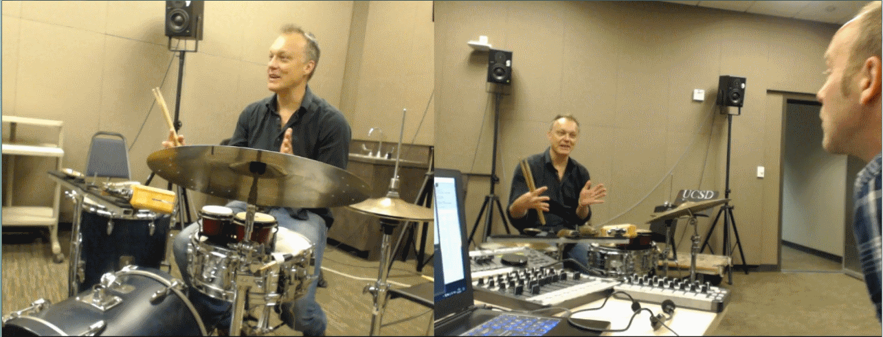
Trumpet and drums

Sound example 1: (Step 1) Trumpet live processed with two different effects, convolution (impulse response from water) and overdrive.

The performer was satisfied with the chosen effects, also because the two were quite different in sound quality. The overdrive was experienced as nice, but he would not like to have it present all the time. We decided to save these effects for later use on trumpet, and be aware of dynamic control on the overdrive.

Sound example 2: (Step 1) Drums live processed with dynamically changing delay and a pitch shift 2 octaves down. The performer found the chosen effects interesting, and the mapping was saved for later use.

Sound example 3: (Step 1) Before entering the analyser and adaptive processing we wanted to try playing together with the effects we had chosen to see if they blended well together. The trumpet player had some problems with hearing the drums during the performance, felt as they were a bit in the background. We found out that the direct sound of the drums was a bit low in the mix, and this was adjusted. We discussed that it is possible to make the direct sound of both instruments louder or softer depending what the performer wants to achieve.

Sound example 4. (Step 2/3) For this example we entered into the analyser using transient density on drums. This was tried out by showing the analyser at the same time as doing an accelerando on drums. This was then set up as an adaptive control from drums on the trumpet. For control, the trumpet player had a suggestion that the more transient density the less convolution effect was added to the trumpet (less send to a convolution effect with a recording of water). The reason for this was that it could make more sense to have more water on slow ambient parts than on the faster hectic parts. At the same time he suggested that the opposite should happen when adding overdrive to the trumpet by transient density meaning that the more transient density the more overdrive on the trumpet. During the first take a reverb was added to the overdrive in order to blend the sound more into the production. It felt like the dynamical control over the effects was a bit difficult because the water disappeared to easily, and the overdrive was introduced to easily. We agreed to fine-tune the dynamical control before doing the actual test that is present as sound example 4.

Sound example 5: For this example we changed roles and enabled the trumpet to control the drums (adaptive processing). We followed a suggestion from the trumpet player and used pitch as an analyses parameter. We decided to use this to control the delay effect on the drums. Low notes produced long gaps between delays, whereas high notes produced small gap between delays. This was maybe not the best solution for getting good dynamical control, but we decide to keep this anyway.

Sound example 6: Cross adaptive performance using the effects and control mappings introduced in example 4 and 5. This was a nice experience for the musicians. Even though it still felt a bit difficult to control it was experienced as musical meaningful. Drummer: “Nice to play a steady grove, and listen to how the trumpet changed the sound of my instrument”.

Vocals and piano

Sound example 7: We had now changed the instrumentation over to vocals and piano, and we started with a performance doing live processing on both instruments. The vocals were processed using two different effects using a delay, and convolution through a recording of small metal parts. The piano was processed using an overdrive and convolution through water.

Sound example 8: Cross adaptive performance where the piano was analysed by rhythmical consonance controlling the delay effect on vocals. The vocal was analysed by transient density controlling the convolution effect on the piano. Both musicians found this difficult, but musically meaningful. Sometimes the control aspect was experienced as counterintuitive to the musical intention. Pianist: It felt like there was a 3rd musician present.

Saxophone self-adaptive processing

Sound example 9: We started with a performance doing live processing to familiarize the performer with the effects. The performer found the augmentation of extended techniques as clicks and pops interesting since this magnified “small” sounds.

Sound example 10: Self-adaptive processing performances where the saxophone was analysed by transient density and then used to control two different convolution effects (recording of metal parts and recording of a cymbal). The first one resulting in a delay effect the second as a reverb. The higher transient density in the analyses the more delay and less reverb and vice versa. The performer experienced the quality of the effects quit similar so we removed the delay effect.

Sound example 11: Self-adaptive processing performances using the same set-up but changing the delay effect to overdrive. The use of overdrive on saxophone did not bring anything new to the table the way it was set up since the acoustic sound of the instrument could sound similar to the effect when putting in strong energy.

Day 2. Wednesday 8 th March

Saxophone and piano

Sound example 12: Performance with saxophone and live processing, familiarizing the performer with the different effects and then choose which of the effects to bring further into the session. Performer found this interesting and wanted to continue with reverb ideas.

Sound example 13: Performance with piano and live processing. The performer especially liked the last part with the delays – Saxophonist: “It was like listening to the sound under water (convolution with water) sometimes, and sometimes like listening to an old radio (overdrive)”. Piano wanted to keep the effects that were introduced.

Sound example 14: Adaptive processing, controlling delay on saxophone from the piano by using analyses of the transient density. The higher transient density, the larger gap between delays on the saxophone. The saxophone player found it difficult to interact since the piano had a clean sound during performance. The piano on the other hand felt in control over the effect that was added.

Sound example 15: Adaptive processing using saxophone to control piano. We analyzed the rhythmical consonance on saxophone. The higher degree of consonance, the more convolution effect (water) was added to piano and vice versa. Saxophone didn’t feel in control during performance, and guessed it was due to not holding a steady rhythm over a longer period. The direct sound of the piano was also a bit loud in the mix making the added effect a bit low in the mix. Piano felt that saxophone was in control, but agreed to the point that the analyses was not able to read to the limit because of the lack of a steady rhythm over a longer time period.

Sound example 16: Crossadptive performance using the same set-up as in example 14 and 15. Both performers felt in control, and started to explore more of the possibilities. Interesting point when the saxophone stops to play since the rhythmical consonance analyses will make a drop as soon as it starts to read again. This could result in strong musical statements.

Sound example 17: Crossadaptive performance keeping the same setting but adding rms analyses on the saxophone to control a delay on the piano (the higher rms the less delay and vice versa).

Vocals and electric guitar

Sound example 18: Performance with vocals and live processing. Vocalist: “It is fun, but something you need to get use to, needs a lot of time”.

Sound example 19: Performance with Guitar and live processing. Guitarist: “Adapted to the effects, my direct sound probably sounds terrible, feel that I`m loosing my touch, but feels complementary and a nice experience”.

Sound example 20: Performance with adaptive processing. Analyzing the guitar using rms and transient density. The higher transient density the more delay added to the vocal, and higher rms the less reverb added to the vocal. Guitar: I feel like a remote controller and it is hard to focus on what I play sometimes. Vocalist: “Feels like a two dimensional way of playing”.

Sound example 21: Performance with adaptive processing. Controlling the guitar by vocals. Analyzing the rhythmical consonance on the vocal to control the time gap between delays inserted on the guitar. Higher rhythmical consonance results in larger gaps and vice versa. The transient density on vocal controls the amount of pitch shift added to the guitar. The higher transient density the less volume is sent to the pitch shift.

Sound example 22: Performance with cross adaptive processing using the same settings as in sound example 20 and 21.

Vocalist: “It is another way of making music, I think”. Guitarist: “I feel control and I feel my impact, but musical intention really doesn’t fit with what is happening – which is an interesting parameter. Changing so much with doing so little is cool”.

Observation and reflections

The sessions has now come to a point were there is less time used on setting up and figuring out how the functionality in the software works, and more time used on actual testing. This is an important step taking in consideration working with musicians that are introduced to the concept the first time. A good stability in software and separation between microphones makes the workflow much more effective. It still took some time to set up everything the first day due to two system crashes, the first one related to the midiator, the second one related to video streaming.

Since preparing the system beforehand there was a lot of reuse both concerning analyzing methods and the choice of effects. Even though there were a lot of reuse on the technical side the performances and results has a large variety in expressions. Even though this is not surprising we think it is an important aspect to be reminded of during the project.

Another technical workaround that was discussed concerning the analyzing stage was the possibility to operate with two different microphones on the same instrument. The idea is then to use one for reading analyses, and one for capturing the “total” sound of the instrument for use in processing. This will of course depend on which analyzing parameter in use, but will surely help for a more dynamical reading in some situations both concerning bleeding, but also for closer focus on wanted attributes.

The pedagogical approach using the four-step introduction was experienced as fruitful when introducing the concept to musicians for the first time. This helped the understanding during the process and therefor resulted in more fruitful discussions and reflections between the performers during the session. Starting with live processing says something about possibilities and flexible control over different effects early in the process, and gives the performers a possibility to be a part of deciding aesthetics and building a framework before entering the control aspect.

Quotes from the the performers:

Guitarist: “Totally different experience”. “Felt best when I just let go, but that is the hardest part”. “It feels like I’m a midi controller”. “… Hard to focus on what I’m playing”. “Would like to try out more extreme mappings”

Vocalist: “The product is so different because small things can do dramatic changes”. “Musical intention crashes with control”. “It feels like a 2-dimensional way of playing”

Pianoist: “Feels like an extra musician”

Live convolution with Kjell Nordeson

Session at UCSD March 14.

Kjell Nordeson: Drums
Øyvind Brandtsegg: Vocals, Convolver.

Contact mikes

In this session, we explore the use of convolution with contact mikes on the drums to reduce feedback and cross-bleed. There is still some bleed from drums into the vocal mike, and there is some feedback potential caused by the (miked) drumheads resonating with the sound coming from the speaker. We have earlier used professional contact mikes, but found that our particular type did have a particularly low output, so this time we tried simple and cheap piezo elements from Radio shack, directly connected to high impedance inputs on the RME soundcard. This seems to give very high sensitivity and a fair signal to noise ratio. The frequency response is quite narrow and “characteristic” to put it mildly, but for our purposes, it can work quite well. Also, the high frequency loss associated with convolution is less of an issue when the microphones have such an abundance of high frequencies (and little or no low end).

IR update triggering

We have added the option of using a (midi) pedal to trigger IR recording. This allows a more deliberate performative control of the IR update. This was  first used by Kjell, while Øyvind was playing through Kjell’s IR. Later switched roles. Kjell notes that the progression from IR to IR works well, and that we definitely have some interesting interaction potential here. The merging of the sound from the two instruments creates a “tail” of what has been played, and that we continue to respond to that for a while.
When Kjell recorded the IR, he thought it was an extra distraction to have to also need to focus on what to record , and to operate the pedal accordingly. The mental distraction probably is not so much in the actual operation of the pedal, but in the reflection over what would make a good sound to record . It is not yet easy to foresee (hear) what comes out of the convolution process, so understanding how a particular input will work as an IR is a sort of remote and second-degree guesswork. This is of course also further complicated by not knowing what the other performer will play through the recorded IR. This will obviously become better with more experience using the techniques.
When we switched roles (vocal recording the IR), the acoustic/technical situation became a bit more difficult. The contact mikes, would pick up enough sound from the speakers (also through freely resonating cymbals resting on the drums, and via non-damped drum heads) to create feedback problems. This also creates extra repetitions of the temporal pattern of the IR due to the feedback potential. It was harder to get the sound completely dry and distinct, so the available timbral dynamic was more in the range from “mushy” to “more mushy” (…). Still, Kjell felt this was “more like playing together with another musician”. The feeling of playing through the IR is indeed the more performatively responsive situation, overpowered by the reduction in clarity that was caused by the technical/acustical difficulties. Similarly, Øyvind thought it was harder because the vocals only manifest themself as the ever changing IR, and the switching if the IR does not necessarily come across as a real/quick/responsive musical interaction. Also, delivering some material for the IR makes the quality of the material and the exact excerpt much more important. It is like giving away some part of what you’ve played, and it must be capable of being transformed out of your own control, so the material might become more transparent to it’s weaknesses. One can’t hide any flaws by stringing the material together in a well-flowing manner, rather the stringing-together is activated by the other musician. Easily, I can recognize this as the situation any musician being live sampled or live processed must feel, so it is a “payback time” revelation for me, having been in the role of processing others for many years.

Automatic IR update

We also tried automatic/periodic IR updates , as that would take the distraction of selecting IR material away, and we could more easily just focus on performing. The automatic updates shows their own set of weaknesses when compared with the manually triggered ones. The automatic update procedure essentually creates a random latency for the temporal patterns created by the convolution. This is because the periodic update is not in any way synchronized to the playing, and the performers do not have a feedback (visually or auditively) on the update pulse. This means the the IR update might happen offbeat or in the middle of a phrase. Kjell suggested further randomizing it as one solution. To this, Øyvind responds that it is already essentially random since the segmentation of input and the implied pulse of the material is unrelated, so it will shift in an unpredictable and always changing manner. Then again, following up on Kjells suggestion and randomizing it further could create a whole other, more statistical approach .  Kjell also remarks that this way of playing it feels more like “an effect”, something added, that does not respond as interactively . It just creates a (echo pattern) tail out of whatever is currently played. He suggested updating the IR at a much lower rate, perhaps once every 10 seconds. We tried a take with this setting too.

Switching who has the trigger pedal

Then, since the automatic updates seems not to work too well, and the mental distracion of selecting IR material seems unwanted, we figured, maybe the musician playing through the IR should be the one triggering the IR recording . This is similar (but exactly opposite) to the previous attempts at manual IR record triggering. Here, the musician playing through the IR is the one deciding the time of IR recording, and as such has some influence over the IR content. Still he can not decide what the other musician is playing at the time of recording , but this type of role distribution could create yet another kind of dynamic in the interplay. Sadly the session was interrupted by practical matters at this point, so the work must continue on a later occation.

Audio


Take1: Percussion IR, vocal playing through the IR. Recording/update of IR done by manual trigger pedal controlled by the percussionist. Thus it is possible to emphasize precise temporal patterns. The recording is done only with contact mikes on the drums, so there is some “disconnectedness” to the acoustic sound.


Take2: Vocal IR, percussion playing through the IR. Recording/update of the IR done by manual trigger pedal controlled by the singer. As in take 1, the drums sound going into the convolver  is only taken from the piezo pickups. Still, there is a better connectedness to the acoustic drum sound, due to an additional room mike being used (dry).


Take3: Percussion IR, automatic/periodic IR update. IR length is 3 seconds, IR update rate is 0.6 Hz.


Take4: Percussion IR, automatic/periodic IR update. IR length is 2.5 seconds, IR update rate is 0.2 Hz.

Other reflections

IR replacement is often experienced as a sudden musical change . There is no artifacts caused by the technical operation of updating the IR, but the musical result is more often a total change of “room characteristic”. Maybe we should try finding methods of slowly crossfading when updating the IR, keeping some aspects of the old one in a transitory phase. There is also a lot to be gained performatively, by the musician updating the IR having these transitions in mind. Choosing what to play and what to record is an effective way of controlling if the transitions should be sudden or slow.

Conversation with Marije, March 2017

After an inspiring talk with Marije on March 3rd, I set out to write this blog post to sum up what we had been talking about. As it happens (and has happened before), Marije had a lot of pointer to other related works and writings. Only after I had looked at the material she pointed to, and reflected upon it, did I get around to writing this blog post. So substantial parts of it contains more of a reflection after the conversation, rather than an actual report of what was said directly.
Marije mentiones we have done a lot of work, it is inspiring, solid, looks good.

Agency, focus of attention

One of the first subjects in our conversation was how we relate to the instrument. For performers: How does it work? Does it work? (does it do what we say/think it does?) What do I control? What controls me? when successful it might constitute a 3rd agency , a shared feeling, mutual control. Not acting as a single musician, but as an ensemble. The same observation can of course be made (when playing) in acoustic ensembles too, but it is connected differently in our setting.

Direct/indirect control . Play music or generate control signals? Very direct and one-dimensional mappings can easily feel like playing to generate control signals. Some control signals can be formed (by analyzing) over longer time spans, as they represent more of a “situation” than an immediate “snapshot”. Perhaps just as interesting for a musician to outline a situation over time , than to simply control one sonic dimension by acting on another?

Out-of-time’d-ness , relating to the different perceptions of the performative role experienced in IR recording (see posts on convolution sessions here, here and here ). A similar experience can be identified within other forms of live sampling. to some degree recognizable with all sorts of live processing as an instrumental activity. For the live processing performer: a detached-ness of control as opposed to directly playing each event.

Contrived and artificial mappings. I asked whether the analyzer-modulation mappings are perhaps too contrived, too “made up”? Marije replying that everything we do with electronic music instrument design (and mapping) is to some degree made up. It is always artibrary, design decisions, something made up. There is not one “real” way, no physical necessity or limitation that determines what the “correct” mapping is. As such, there are only mappings that emphasize different aspects of performance and interaction, new ideas that might seem “contrived” can contain yet-to-be-seen areas of such emphasis. Composition is in these connections. For longer pieces one might want variation in mapping. For example, in the combined instrument created by voice and drums in some of our research sessions. Depending on combination and how it is played, the mapping might wear out over time, so one might want to change it during one musical piece.

Limitation. In January I did a presentation at UC Irvine, for an audience well trained in live processing and electronic music performance. One of the perspectives mentioned there was that the cross-adaptive mapping could also be viewed as a limitation. One could claim that all of these modulations that we can perform cross-adaptively could have been manually controlled, an with much more musical freedom if manually controlled. Still, the crossadaptive situation provides another kind of dynamic . The acoustic instrument is immediate and multidimensional, providing a nuanced and intuitive interface. We can tap into that. As an example as to how the interfacne changes the expression, look at how we (Marije) use accelerometers over 3 axes of motion: one could produce the same exact same control signals using 3 separate faders, but the agency of control , the feeling, the expressivity, the dynamic is different with accelerometers that it is with faders. It is different to play , and this will produce different results. The limitations (of an interface or a mapping) can be viewed as something interesting, just as much as something that inhibits.

Analyzer noise and flakyness

One thing that have concerned me lately is the fact that the analyzer is sometimes too sensitive to minor variations in the signal. Mathematical differences sometimes occur on a different scale than the expressive differences . One example is the rhythm analyzer, the way I think it is too noisy and unreliable, seen in the light of the practical use in session , where the musicians found it very appropriate and controllable.
Marije reminds me that in the live performance setting, small accidents and surprises are inspiring. In a production setting perhaps not so much. Musicians are trained to embrace the imperfections of, and characteristic traits of their instument, so it is natural for them to also respond in a similar manner to imperfections in the adaptive and crossadaptive control methods. This makes me reflect if there is a research methodology of accidents(?), on how to understand the art of the accident, understand the failure of the algorithm, like in glitch, circuit bending, and other art forms relating to distilling and refining “the unwanted”.

Rhythm analysis

I will refine the rhythm analysis, it seems promising as a measure
of musical expressivity. I have some ideas of maintaining several parallel hypotheses on how to interpret input, based on previous rhythm research. some of this comes from “Machine Musicianship” by Robert Rowe, some from readin a UCSD dissertation by Michelle L. Daniels: “An Ensemble Framework for Real-Time Beat Tracking”. I am currently trying to distill these into a simplest possible method of rhythm analysis for our purposes. So I ask Marije on ideas on how to refine the rhythm analyzer. Rhythm can be one parameters that outlines “a situation” just as much as it creates a “snapshot” (recall the discussion of agency and direct/indirect control, above). One thing we may want to extract is slower shifts, from one situation to another. My concerns that it takes too long to analyze a pattern (well, at least as long as the pattern itself, which might be several seconds) can then be regarded less of a concern, since we are not primarily looking for immediate output. Still, I will attempt to minimize the latency of rhythm analysis, so that any delay in response is due to aestethic choice, and not so much limited by the technology. She also mentions the other Nick Collins. I realize that he’s the one behind the bbcut algorithm also found in Csound. I’ve used a lot a long time ago. Collins has written a library for feature extraction within SuperCollider. To some degree there is overlap with feature extraction on our Analyzer plugin. Collins invokes external programs to produce similarity matrices , something that might be useful for our purposes as well, as a means of finding temporal patterns in the input. In terms of rhythm analysis, it is based on beat tracking as is common. While we in our rhythm analysis attempts at *not relying* on beat tracking, we could still perhaps implement it, if nothing else so to use it as a measure of beat tracking confidence (assuming this as a very coarse distinction between beat based and more temporally free music.
Another perspective on rhythm analysis can also perhaps be gained from Clarence Barlow’s interest in ratios. The ratio book is available online, as is a lot of his other writings .  Barlow states “In the case of ametric music, all pulses are equally probable”… which leads me to think that any sort of statistical analysis, frequency of occurence of observed inter-onset times, will start to give indications of “what this is”… to lift it slowly out of the white-noise mud of equal probabilities.

Barlow uses the “ Indispensability formula “, for relating the importance of each subdivision within a given meter. Perhaps we could invert this somehow to give a general measure of “ subdivided-ness “?. We’re not really interested in finding the meter, but the patterns of subdivision is nonetheless of interest. He also use the “ Indigestibility formula ” for ratios, based on prime-ness, suggests also a cultural digestability limit around 10 (10:11, 11:12, 12:13 …). I’ve been pondering different ways of ordering the complexity of different integer ratios, such as different trhythmic subdivisions. The indigesibility formula might be one way to approach it, but reading further in the ratio book, the writing of Demetrios E. Lekkas leads me to think of another way to sort the subdivisions into increasing complexity:

Lekkas describes the traditional manner of writing down all rational numbers by starting with 1/1 (p 38), then increasing the numerator by one, then going through all denominators from 1 up to the nominator, skipping fracions that can be simplified since they represent numbers earlier represented. This ordering does not imply any relation to complexity of the ratios produced. If tried to use it as such, one problem with this ordering is that it determines that subdividing in 3 is less complex than subdividing in 4. Intuitively, I’d say a rhythmic subdivision in 3 is more complex than a further subdivision of the first established subdivision in 2. Now, could we, to try to find a measure of complexity, assume that divisions further apart from any previous established subdivision are simpler than the ones creating closely spaced divisions(?). So, when dividing 1/1 in 2, we get a value at 0.5 (in addition to 0.0 and 1.0, which we omit for brevity). Then, trying to decide what is the next further division is the most complex, we try out all possible further subdivision up to some limit, look at the resulting values and their distances to already excisting values.
Dividing in 3 give 0.33 and 0.66 (approx), while dividing in 4 give the (new) values 0.25 and 0.75. Dividing by 5 gives new values at .2 and .4, by 6 is unnecessary as it does not produce any larger distances than already covered by 3. Divide by 7 gives values at .142, 0.285 and .428. Divide by 8 is unnecessary as it does not produce any values of larger distance than the divide by 4.
The lowest distance introduced by dividing in 3 is 0.33 to 0.5, a distance of approx 0.17. The lowest distance introduced by dividing in 4 is from 0.25 to 0.5, a distance of 0.25. Dividing into 4 is thus less complex. Checking the divide by 5 and 7 can be left as an exercise to the reader.
Then we go on to the next subdivision, as we now have a grid of 1/2 plus 1/4, with values at 0.25, 0.5 and 0.75. The next two alternatives (in increasing numeric order) is division by 3 or division by 5. Division by 3 gives a smallest distance (to our current grid) from 0.25 to 0.33 = 0.08. Division by 5 gives a smallest distance from 0.2 to 0.25 = 0.05. We conclude that division by 3 is less complex. But wait, let’s check division by 8 too while we’re at it also here, leaving divide by 6 and 7 as an exercise to the reader). Division by 8, in relation to our current grid (.25, .5, .75) gives a smallest distance of 0.125. This is larger than the smallest distance produced by division in 3 (0.08), so we choose 8 as our next number in increasing order of complexity.
Following up on this method, using a highest subdivision of 8, eventually gives us this order 2,4,8,3,6,5,7 as subdivisions in increasing order of complexity. This coincides with my intuition of rhythmic complexity , and can be reached by the simple procedure outlined above. We could also use the same procedure to determine the exact value of complexity for each of these subdivisions, as a means to create an output “value of complexity” for integer ratios. As a side note to myself, check how this will differ from using Tenney height or Benedetti height as I’ve used earlier in the Analyzer.

On the justification for coming up with this procedure I might lean lightly on Lekkas again: “If you want to compare them you just have to come up with your own intuitive formula…deciding which one is more important…That would not be mathematical. Mind you, it’s non-mathematical, but not wrong.” (Ratio book p 40)
Much of the book relates to ratios as in pitch ratios and tuning . Even though we can view pitch and rhythm as activity within the same scale, as vibrations/activations at different frequencies, the perception of pitch is further complicated by the anatomy of our inner ear (critical bands), and by cultural aspects and habituation . Assumedly, these additional considerations should not be used to infer complexity of rhythmic activity. We can not directly use harmonicity of pitch as a measure of the harmonicity of rhythm , even though it might *to some extent* hold true (and I have used this measure up until now in the Analyzer).

Further writings by Barlow on this subject can also be found in his On Musiquantics . “Can the simplicity of a ratio be expressed quantitatively?” (s 38), related to the indegestability formula. See also how “metric field strength”  (p 44), relates to the indispensability formula. The section from p 38-47 concerns this issue, as well as his “Formulæ for Harmonicity” p 24, (part II), with Interval Size, Ratios and Harmonic Intensity on the following pages. For pitch, the critical bandwidth (p 48) is relevant but we could discuss if not the “larger distance created by a subdivision” as I outlined above is more appropriate for rhythmic ratios.

Instrumentality

The 3Dmin book “ Musical Instruments in the 21st Century ” explores various notions of what an instrument can be, for example the instrument as a possibility space . Lopes/Hoelzl/de Campo, in their many-fest “favour variety and surprise over logical continuation” and “enjoy the moment we lose control and gain influence”. We can relate this to our recent reflections on how performers in our project thrive in a setting where the analysis meethods are somewhat noisy and chaotic. The essence being they can control the general trend of modulation , but still be surprised and disturbed” by the immediate details. Here we again encounter methods of the “less controllable”: circuit bending, glitch, autopoietic (self-modulating) instruments, meta-control techniques (de Campo), and similarly the XY interface for our own Hadron synthesizer, to mention a few apparent directions. The 3DMIN book also has a chapter by Daphna Naphtali on using live processing as an instrument . She identifies some potential problems about the invisible instrument . One problem, according to Naptali, is that it can be difficult to identify the contribution (of the performer operating it). One could argue that invisibility is not necessarily a problem(?), but indeed it (invisibility and the intangible) is a characteristic trait of the kind of instruments that we are dealing with, be it for live processing as controlled by an electronnic musician, or for crossadaptive processing as controlled by the acoustic musicians.

Marije also has a chapter in this book, on the blurring boundaries between composition, instrument design, and improvisation. …”the algorithm for the translation of sensor data into music control data is a major artistic
area; the definition of these relationships is part of the composition of a piece” Waisvisz 1999 , cited by Marije

Using adaptive effects as a learning strategy

In light of the complexity of crossadaptive effects, the simpler adaptive effects could be used as a means of familiarization for both performers and “mapping designers” alike. Getting to know how the analyzer reacts to different source material, and how to map the signals in a musically effective manner. The adaptive use case is also more easily adaptable to a mixing situation, for composed music, and any other kind of repeatable situation. The analyzer methods can be calibrated and tuned more easily for each specific source instrument. Perhaps we could also look at a possible methodology for familiarization , how do we most efficiently learn to know these feature-to-modulator mappings. Revising the literature on adaptive audio effects (Verfaille etc) in the light of our current status and reflections might be a good idea.

Performers utilizing adaptive control

Similarly, it might be a good idea to get on touch with environments and performers using adaptive techniques as part of their setup. Marije reminded me that Jos Zwaanenburg and his students at the Conservatorium of Amsterdam might have more examples of musicians using adaptive control techniques. I met Jos some years ago, and contacted him again via email now. Hans Leeouw is another Dutch performer working with adaptive control techniques.  His 2009 NIME article mentions no adaptive control, but has a beautiful statement on the design of mappings: “…when the connection between controller and sound is too obvious the experience of ‘hearing what you see’ easily becomes ‘cheesy’ and ‘shallow’. One of the beauties of acoustic music is hearing and seeing the mastery of a skilled instrumentalist in controlling an instrument that has inherent chaotic behaviour “. In the 2012 NIME article he mentions audio analyses for control. I Contacted Hans to get more details and updated information about what he is using. Via email he tells that he use noise/sinusoidal balance as a control both for signal routing (trumpet sound routed to different filters), and also to reconfigure the mapping of his controllers (as appropriate for the different filter configuration). He mentions that the analyzed transition from noise to sinusoidal can be sharp, and that additional filtering is needed to geet a smooth transition. A particularly interesting area occurs when the routing and mapping is in this intermediate area, where both modes of processing and mapping are partly in effect.

As an example of on researcher/performer that has explored voice control, Marije mentioned Dan Stowell .
Nor surprisingly, he’s also done his research in the context of QMUL. Browsing his thesis, I note some useful terms for ranking extracted features, as he writes about * perceptual relevance *, * robustness *, and * independence *. His experiments on ranking the different features are not conclusive, as “none of the experiments in themselves will suggest a specific compact feature set”. This indication coincides with our own experience so far as well, that different instruments and different applications require different subsets of features. He does however mention spectral centroid, to be particularly useful . We have initially not used this so much due to a high degree of temporal fluctuation. Similarly, he mentions spectral spread , where we have so far used more spectral flatness and spectral flux . This also reminds me of recent discussions on the Csound list regarding different implementations of the analysis of spectral flux (difference from frame to frame or normalized inverse correlation), it might be a good idea to test the different implementations to see if we can have several variations on this measure, since we have found it useful in some but not all of our application areas. Stowell also mentions log attack time , which we should revisit and see how we can apply or reformulate to fit our use cases. A measure that we haven’t considered so far is delta MFCCs , the temporal variation within each cepstral band. Intuitively it seems to me this couldd be an alternative to spectral flux, even though Stowell have found it not to have a significant mutual information bit (delta MFCC to spectral flux). In fact the Delta MFCCs have little MI with any other features whatsoever, although this could be related to implementation detail (decorrelation). He also finds that Delta MFCC have low robustness, but we should try implementing it and see what it give us. Finally, he also mentions * clarity * as a spectral measure, in connectino to pitch analysis, defined as “ the normalised strength of the second peak of the autocorrelation trace [McLeod and Wyvill, 2005]”. It is deemed a quite robust measure, and we could most probably implement this with ease and test it.

Seminar: Mixing and timbral character

Online conversation with Gary Bromham (London), Bernt Isak Wærstad (Oslo), Øyvind Brandtsegg (San Diego), Trond Engum and Andreas Bergsland (Trondheim). Gyrid N. Kaldestad, Oslo, was also invited but unable to participate.

The meeting revolves around the issues “mixing and timbral character” as related to the crossadaptive project. As there are many aspects of the project that touches upon these issues, we have kept the agenda quite open as of yet, but asking each participant to bring one problem/question/issue.

Mixing, masking

In Oslo they worked with the analysis parameters spectral crest and flux, aiming to use these to create a spectral “ducking” effect, where the actions of one instrument could selectively affect separate frequency bands of the other instrument. Gary is also interested in these kinds of techniques for mixing, to work with masking (allowing and/or avoiding masking). One could think if it as a multiband sidechaining with dynamic bands, like a de-esser, but adaptive to whichever frequency band currently needs modification. These techniques are related both to previous work on adaptive mixing (for example at QMUL) and also partially solved by recent commecial plugins, like Izotope Neutron .
However interesting these techniques are, the main focus of our current project is more on the performative application of adaptive and crossadaptive effects. That said, it could be fruitful using these techniques, not to solve old problems, but to find new working methods in the studio as well. In the scope of the project, this kind of creative studio work can be aimed at familiarizing ourselves with the crossadaptive methods in a controlled and repeatable setting. Bernt also brought up the issue of recording the analysis signals, using them perhaps as source material for creative automation, editing the recorded automation as one might see fit. This could be an effective way of familiarization with the analyzer output as well, as it invites taking a closer look at the details of the output of the different analysis methods. Recording the automation data is straightforward in any DAW, since the analyzer output comes into the DAW as external MIDI or OSC data. The project does not need to develop any custom tools to allow recording and editing of these signals, but it might be a very useful path of exploration in terms of working methods. I’d say yes please, go for it.

Working with composed material, post production

Trond had recently done a crossadaptive session with classical musicians, playing composed material. It seems that this, even though done “live” has much in common with applying crossadaptive techniques in post production or in mixing. This is because the interactive element is much less apparent. The composition is a set piece, so any changes to the instrumental timbre will not change what is played , but rather can influence the nuances of interpretation. Thus, it is much more a one-way process instead of a dialectic between material and performance. Experts on interpretation of composed music will perhaps cringe at this description, saying there is indeed a dialogue between interpretation and composition. While this is true, the degree to which the performed events can be changed is lesser within a set composition. In recent sessions, Trond felt that the adaptive effects would exist in a paralell world, outside of the composition’s aesthetic, something unrelated added on top . The same can be said about using adaptive and crossadaptive techniques in a mixing stage of a production, where all tracks are previously recorded and thus in a sense can be regarded as a set (non-changeable) source. With regards to applying analysis and modulation to recorded material, one could also mention that the Oslo sessions used recordings of the (instruments in the session) to explore the analysis dimensions. This was done as an initial exploratory phase of the session. The aim was finding features that already exist in the performer’s output, rather than imposing new dimensions of expression that the performer will need to adapt to.

On repeatability and pushing the system

The analysis-modulator response to an acoustic input is not always explicitly controllable. This is due to the nature of some of the analysis methods, technical weaknesses that introduce “flicker” or noise in the analyzer output. Even though these deviations are not inherently random, they are complex and sometimes chaotic. In spite of these technical weaknesses, we notice that our performers often will thrive. Musicians will often “go with the flow” and create on the spot, the interplay being energized by small surprises and tensions, both in the material and in the interactions. This will sometimes allow the use of analysis dimensions/methods that have spurious noise/flicker, still resulting in a consistent and coherent musical output, due to the performer’s experience in responding to a rich environment of sometimes contradicting signals. This touches one of the core aspects of our project, intervention into the traditional modes of interplay and musical communication . It also touches upon the transparency of the technology, how much should the performer be aware of the details of the signal chain? Sometimes rationalization makes us play safe. A fruitful scenario would be aiming for analysis-modulator mappings that create tension, something that intentionally disturbs and refreshes. The current status of our research leaves us with a seemingly unlimited amount of combinations and mappings, a rich field of possibilities, yet to be charted. The options are still so many that any attempt at conclusions about how it works or how to use it seems futile. Exploration in many directions is needed. This is not aimless exploration, but rather searching without knowing what can be found.

Listening, observing

Andreas mentions is is hard to pinpoint single issues in this rich field. As observer it can be hard to decode what is happening in the live setting. During sessions, it is sometimes a complex task following the exact details of the analysis and modulation. Then, when listening to the recorded tracks again later, it is easier to appreciate the musicality of the output. Perhaps not all details of the signal chain are cleanly defined and stringent in all aspects, but the resulting human interaction creates a lively musical output. As with other kinds of music making, it is easy to get caught up in detail at time of creation. Trying to listen more in a holistic manner, taking in the combined result, is a skill not to be forgotten also in our explorations.

Adaptive vs cross-adaptive

One way of working towards a better understanding of the signal interactions involved in our analyzer-modulator system is to do adaptive modulation rather than cross-adaptive. This brings a much more immediate mode of control to the performer, exploring how the extracted features can be utilized to change his or her own sound. It seems several of us have been eager to explore these techniques, but putting it off since it did not align with the primary stated goals of crossadaptivity and interaction. Now, looking at the complexity of the full crossadaptive situation, it is fair to say that exploration of adaptive techniques can serve as a very valid manner of getting in touch with the musical potential of feature-based modulation of any signal. In it’s own right, it can also be a powerful method of sonic control for a single performer, as an alternative to a large array of physical controllers (pedals, faders, switches). As mentioned earlier in this session, working with composed material or set mixes can be a challenge to the crossadaptive methods. Exploring adaptive techniques might be more fruitful in those settings. Working with adaptive effects also brings the attention to other possibilities of control for a single musician over his or her own sound. Some of the recent explorations of convolution with Jordan Morton shows the use of voice controlled crossadaptivity as applied to a musician’s own sound. In this case, the dual instrument of voice and bass operated by a single performer allows similar interactions between instruments, but bypassing the interaction between different people, thus simplifying the equation somewhat. This also brings our attention to using voice as a modulator for effects for instrumentalists not using voice as part of their primary musical output. Although this has been explored by several others (e.g. Jordi Janner , Stefano Fasciani , and also the recent Madrona Labs “Virta” synth ) it is a valid and interesting aspect, integral to our project.

Convolution experiments with Jordan Morton

Jordan Morton is a bassist and singer, she regularly performs using both instruments combined. This provides an opportunity to explore how the liveconvolver can work when both the IR and the live input are generated by the same musician. We did a session at UCSD on February 22nd. Here are some reflections and audio excerpts from that session.

General reflections

As compared with playing with live processing, Jordan felt it was more “up to her” to make sensible use of the convolution instrument. With live processing being controlled by another musician, there is also a creative input from another source. In general, electronic additions to the instrument can sometimes add unexpected but desirable aspects to the performance. With live convolution where she is providing both signals, there is a triple (or quadruple) challenge: She needs to decide what to play on the bass, what to sing, explore how those two signals work together when convolved, and finally make it all work as a combined musical statement. It appears this is all manageable, but she’s not getting much help from the outside. In some ways, working with convolution could be compared to looping and overdubs, except the convolution is not static. One can overlay phrases and segments by recording them as IR’s, while shaping their spectral and temporal contour with the triggering sound (the one being convolved with the IR).
Jordan felt it easier to play bass through the vocal IR than the other way around . She tend to lead with the bass when playing acoustic on bass + vocals. The vocals are more an additional timbre added to complete harmonies etc with the bass providing the ground. Maybe the instrument playing through the IR has the opportunity of more actively shaping the musical outcome, while the IR record source is more a “provider” of an environment for the other to actively explore?
In some ways it can seem easier to manage the roles roles (of IR provider and convolution source) as one person than splitting the incentive among two performers. The roles becomes more separated when they are split between different performers than when one person has both roles and then switches between them. When having both roles, it can be easier to explore the nuances of each role. Possible to test out musical incentives by doing this here and then this there , instead of relying on the other person to immediately understand (for example to *keep* the IR, or to *replace* it *now* ).

Technical issues

We explored transient triggered IR recording, but had a significant acoustic bleed from bass into the vocal microphone, which made clean transient trigging a bit difficult. A reliable transient triggered recording would be very convenient, as it would allow the performer to “just play”. We tried using manual triggering, controlled by Oeyvind. This works reliably but involves some guesswork as to what is intended to be recorded. As mentioned earlier (e.g. in the first Olso session ), we could wish for a foot pedal trigger or other controller directly operated by the performer. Hey it’s easy to do, let’s just add one for next time.
We also explored continuous IR updates based on a metronome trigger. This allows periodic IR updates, in a seemingly streaming fashion. Jordan asked for an indication of the metronomic tempo for the updates, which is perfectly reasonable and would be a good idea to do (although had not been implemented yet). One distinct difference noted when using periodic IR updates is that the IR is always replaced. Thus, it is not possible to “linger” on an IR and explore the character of some interesting part of it. One could simulate such exploration by continuously re-recording similar sounds, but it might be more fruitful to have the ability to “hold” the IR, preventing updates while exploring one particular IR. This hold trigger could reasonably also be placed on a footswitch or other accessible control for the performer.

Audio excerpts


Take 1: Vocal IR, recording triggered by transient detection.


Take 2: Vocal IR, manually triggered recording


Take 3: Vocal IR, periodic automatic trigger of IR recording.


Take 4: Vocal IR, periodic automatic trigger of IR recording (same setup as for take 3)


Take 5: Bass IR, transient triggered recording. Transient triggering worked much cleaner on the bass since there was less signal bleed from voice to bass than vice versa.