Exploring radically new modes of musical interaction in live performance
Category: Sessions
Session with Kim Henry Ortveit
February 22, 2018
-
Kim Henry is currently a master student at NTNU music technology, and as part of his master project he has designed a new hybrid instrument. The instrument allows close interactions between what is played on a keyboard (or rather a ...
Session with Michael Duch
February 22, 2018
-
February 12th, we did a session with Michael Duch on double bass, exploring auto-adaptive use of our techniques. We were interested in seeing how the crossadaptive techniques could be used for personal timbral expansion for a single player. This is ...
Session with David Moss in Berlin
February 2, 2018
-
Thursday February 1st, we had an enjoyable session at the Universität der Kunste in Berlin. This was at the Grunewaldstraße campus and generously hosted by professor Alberto De Campo. This was a nice opportunity to follow up on earlier collaboration ...
Session with 4 singers, Trondheim, August 2017
October 9, 2017
-
Location: NTNU, Studio Olavshallen. Date: August 28 2017 Participants: Sissel Vera Pettersen, vocals Ingrid Lode, vocals Heidi Skjerve, vocals Tone Åse, vocals Øyvind Brandtsegg, processing Andreas Bergsland, observer and video documentation Thomas Henriksen, sound engineer Rune Hoemsnes, sound engineer We ...
Session in UCSD Studio A
September 8, 2017
-
This session was done May 11th in Studio A at UCSD. I wanted to record some of the performer constellations I had worked with in San Diego during Fall 2016 / Spring 2017. Even though I had worked with all ...
Session with Jordan Morton and Miller Puckette, April 2017
June 9, 2017
-
This session was conducted as part of preparations to the larger session in UCSD Studio A, and we worked on calibration of the analysis methods to Jordans double bass and vocals. Some of the calibration and accomodation of signals also includes ...
Liveconvolver experiences, San Diego
June 7, 2017
-
The liveconvolver has been used in several concerts and sessions in San Diego this spring. I played three concerts with the group Phantom Station (The Loft, Jan 30th, Feb 27th and Mar 27th), where the first involved the liveconvolver. Then ...
Live convolution session in Oslo, March 2017
June 7, 2017
-
Participants: Bjørnar Habbestad (flute), Bernt Isak Wærstad (guitar), Gyrid Nordal Kaldestad (voice) Mats Claesson (documentation and observation). The focus for this session was to work with the new live convolver in Ableton Live Setup - getting to know the Convolver We ...
Second session at Norwegian Academy of Music (Oslo) – January 13. and 19., 2017
June 7, 2017
-
Participants: Bjørnar Habbestad (flute), Bernt Isak Wærstad (guitar), Gyrid Nordal Kaldestad (voice) The focus for this session was to play with, fine tune and work further on the mappings we sat up during the last session at NMH in November. Due ...
Cross adaptive session with 1st year jazz students, NTNU, March 7-8
April 6, 2017
-
This is a description of a session with first year jazz students at NTNU recorded March 7 and 8. The session was organized as part of the ensemble teaching that is given to jazz students at NTNU, and was meant to take care ...
Live convolution with Kjell Nordeson
March 23, 2017
-
Session at UCSD March 14. Kjell Nordeson: Drums Øyvind Brandtsegg: Vocals, Convolver. Contact mikes In this session, we explore the use of convolution with contact mikes on the drums to reduce feedback and cross-bleed. There is still some bleed from ...
Session with classical percussion students at NTNU, February 20, 2017
March 10, 2017
-
Introduction: This session was a first attempt in trying out cross-adaptive processing with pre-composed material. Two percussionists, Even Hembre and Arne Kristian Sundby, students at the classical section, were invited to perform a composition written for two tambourines. The musicians ...
Convolution experiments with Jordan Morton
March 1, 2017
-
Jordan Morton is a bassist and singer, she regularly performs using both instruments combined. This provides an opportunity to explore how the liveconvolver can work when both the IR and the live input are generated by the same musician. We did a ...
Docmarker tool
February 16, 2017
-
Docmarker During our studio sessions and other practical research work sessions, we noted that we needed a tool to annotate documentation streams. The stream could be an audio file, a video or some line of timed events. Audio editors and ...
Session UCSD 14. Februar 2017
February 15, 2017
-
Session objective The session objective was to explore the live convolver, how it can affect our playing together and how it can be used. New convolver functionality for this session is the ability to trigger IR update via transient detection, ...
Crossadaptive session NTNU 12. December 2016
December 16, 2016
-
Participants: Trond Engum (processing musician) Tone Åse (vocals) Carl Haakon Waadeland (drums and percussion) Andreas Bergsland (video) Thomas Henriksen (sound technician) Video digest from session: https://www.youtube.com/watch?v=ktprXKVdqF4&feature=youtu.be Session objective and focus: The main focus in this session was to explore other ...
Oslo, First Session, October 18, 2016
December 12, 2016
-
First Oslo Session. Documentation of process 18.11.2016 Participants Gyrid Kaldestad, vocal Bernt Isak Wærstad, guitar Bjørnar Habbestad, flute Observer and Video Mats Claesson The Session took place in one of the sound studios at the Norwegian Academy of Music, Oslo ...
Multi-camera recording and broadcasting
November 21, 2016
-
Audio and video documentaion is often an important component of projects that analyse or evaluate musical performance and/or interaction. This is also the case in the Cross Adaptive project where every session was to be recorded in video and multi-track ...
Session 19. October 2016
October 31, 2016
-
Location: Kjelleren, Olavskvartalet, NTNU, Trondheim Participants: Maja S. K. Ratkje, Siv Øyunn Kjenstad, Øyvind Brandtsegg, Trond Engum, Andreas Bergsland, Solveig Bøe, Sigurd Saue, Thomas Henriksen Session objective and focus Although the trio BRAG RUG has experimented with crossadaptive techniques in rehearsals and ...
Session 20. – 21. September
September 30, 2016
-
Location: Studio Olavskvartalet, NTNU, Trondheim Participants: Trond Engum, Andreas Bergsland, Tone Åse, Thomas Henriksen, Oddbjørn Sponås, Hogne Kleiberg, Martin Miguel Almagro, Oddbjørn Sponås, Simen Bjørkhaug, Ola Djupvik, Sondre Ferstad, Björn Petersson, Emilie Wilhelmine Smestad, David Anderson, Ragnhild Fangel Session objective and focus: This post is a description of a session with 3rd year Jazz students at NTNU. It was the first session following the intended procedure ...
Mixing with Gary
June 16, 2016
-
During our week in London we had some sessions with Gary Bromham, first at the Academy of Contemporary Music in Guildford on the June 7th , then at QMUL later in the week. We wanted to experiment with cross-adpative techniques ...
Mixing example, simplified interaction demo
May 24, 2016
-
When working further with some of the examples produced in an earlier session , I wanted to see if I could demonstrate the influence of one instrument's influence of the the other instruments sound more clearly. Here' I've made an example where the ...
Introductory session NTNU, Trond/Øyvind
May 13, 2016
-
Date: 3 May 2016 Location: NTNU Mustek Participants: Trond Engum, Øyvind Brandtsegg Session objective and focus: Test ourselves as musicians in cross adaptive setting. MEaning, test how we react to being in the role of the processed Test out different mappings, ...
Introductory session, NTNU, Bernt/Øyvind
May 13, 2016
-
Date: 26 April 2016 Location: NTNU Mustek Participants: Bernt Isak Wærstad, Øyvind Brandtsegg Session objective and focus: Test ourselves as musicians in cross adaptive setting. We have usually been the processing musicians, now we should test ourselves as the victims ...
Westerdal session April 2016
May 13, 2016
-
Session at Westerdal ACT, OSLO Participants: Ylva Øyen Brandtsegg, Øyvind Brandtsegg Objective: Studio use of cross_shimmer effect Takes Take 1: Cross_shimmer: Vocals as spectral input, Drumset as exciter Take2: As above, another take on the same musical goal Comments: * Feedback not ...
Tape to zero 2016
May 13, 2016
-
Concert : Tape to zero festival, April 21 2016, Victoria Jazz, Nasjonal jazzscene Oslo Participants: Maja S.K. Ratkje, Siv Øyunn Kjenbstad, Øyvind Brandtsegg The objective, in the context of this research project, was live use of the "cross_shimmer" effect, testing musical applications ...
Jazz ensemble, spring 2016
May 13, 2016
-
Experimental session in the context of ensemble teaching at the jazz dept at NTNU, April 2016. The objective was to test some simple interaction modes, starting with cross adaptive amplitude control. How will the musicians react to this kind of interaction? ...
The main focus in this session was to explore other analysing methods than used in earlier sessions (focus on rhythmic consonance for the drums, and spectral crest on the vocals). These analysing methods were chosen to get a wider understanding of their technical functionality, but also their possible use in musical interplay. In addition to this there was an intention to include the sample/hold function for the MIDIator plug-in. The session was also set up with a large screen in the live room to monitor the processing instrument to all participants at all times. The idea was to democratize the processing musician role during the session to open up for discussion and tuning of the system as a collective process based on a mutual understanding. This would hopefully communicate a better understanding of the functionality in the system, and how the musicians individually can navigate within it through their musical input. At the same time this also opens up for a closer dialog around choice of effects and parameter mapping during the process.
Earlier experiences and process
Following up on experiences documented through earlier sessions and previous blog posts, the session was prepared to avoid the most obvious shortcomings. First of all, separation between instruments to avoid bleeding through microphones was arranged by placing vocals and drums in separate rooms. Bleeding between microphones was earlier affecting both the analysed signals and effects. The system was prepared to be as flexible as possible beforehand containing several effects to map to, flexibility in this context meaning the possibility to do fast changes and tuning the system depending on the thoughts from the musicians. Since the group of musicians remained unchanged during the session this flexibility was also seen as a necessity to go into details and more subtle changes both in the MIDIator and the effects in play to reach common aesthetical intentions.
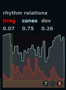
Due to technical problems in the studio (not connected with the cross adaptive set up or software) the session was delayed for several hours resulting in shorter time than originally planned. We therefore made a choice to concentrate only on rhythmic consonance (referred to as rhythmical regularity in the video) as analysing method for both drums and vocals. The method we used to familiarize with this analysing tool was that we started with drums trying out different playing techniques with both regular and irregular strokes while monitoring the visual feedback from the analyser plug-in without any effect. Regular strokes in this case resulting in high stable value, irregular strokes resulting in low value.
Figure 1. Consonance (regularity) visualized in the upper graph.
What became evident was that when the input stopped, the analyser stayed at the last measured value, and in that way could act as a sort of sample/hold function on the last value and in that sense stabilise a setting in an effect until an input was introduced again. Another aspect was that the analysing method worked well for regularity in rhythm, but had more unpredictable behaviour when introducing irregularity.
After learning the analyser behaviour this was further mapped to a delay plugging as an adaptive effect on the drums. The parameter controlled the time range of 14 delays resulting in larger delay time range the more regularity, and vice versa.
After fine-tuning the delay range we agreed that the connection between the analyser, MIDIator and choice of effect worked musically in the same direction. (This was changed later in the session when trying out cross-adaptive processing).
The same procedure was followed when trying vocals, but then concentrating the visual monitoring mostly on the last stage of the chain, the delay effect. This was experienced as more intuitive when all settings were mapped since the musician then could interact visually with the input during performance.
Cross-adaptive processing.
When starting the cross-adaptive recording everyone had followed the process, and tried out the chosen analysing method on own instruments. Even though the focus was mainly on the technical aspects the process had already given the musicians the possibility to rehearse and get familiar with the system.
The system we ended up with was set up in the following way:
Both drums and vocals was analysed by rhythmical consonance (regularity). The drums controlled the send volume to a convolution reverb and a pitch shifter on the vocals. The more regular drums the less of the effects, the less regular drums the more of the effects.
The vocals controlled the time range in the echo plugin on the drums. The more regular pulses from the vocal the less echo time range on the drums, the less regular pulses from the vocals the larger echo time range on the drums.
Sound example (improvisation with cross adaptive setup):
The Session took place in one of the sound studios at the Norwegian Academy of Music, Oslo , Norway
Gyrid Kaldestad (vocal) and Bernt Isak Wærstad (guitar) had one technical/setup meeting beforehand, and there were numerous emails going back and forth before the session that was about technical issues.
Bjørnar Habbestad (flute) where invited into the session.
The observer, decided to make a video documentation of the session.
I’m glad I did because I think it gives a good insight off the process. And a process it was!
The whole session lasted almost 8 hours and it was not until the very last 30 minutes that playing started.
I am (Mats Claesson) not going to comment on the performative musical side of the session. The only reason for this is that the music making happend at the very end of the session, was very short and it was not recorded so I could evaluate it “in depth” However, just watch the comments, from the participants, at the end of the video. They are very positive…..
I think from the musicians side it was rewarding and highly interesting. I am confident that the next session will generate an musical outcome that is substantial enough to be comment on, from both a performative and a musical side.
In the video there are no processed sound of the very last playing due to use of headphone, but you can listen to excerpts posted below the video.
Here is a link to the video
Reflections on the process given from the perspective of the musicians:
We agreed to make a limited setup to have better control over the processing. Starting with basic sounds and basic processing tools so that we easier could control the system in a musical way. We started with a tuning analysis for each instrument (voice, flute, guitar)
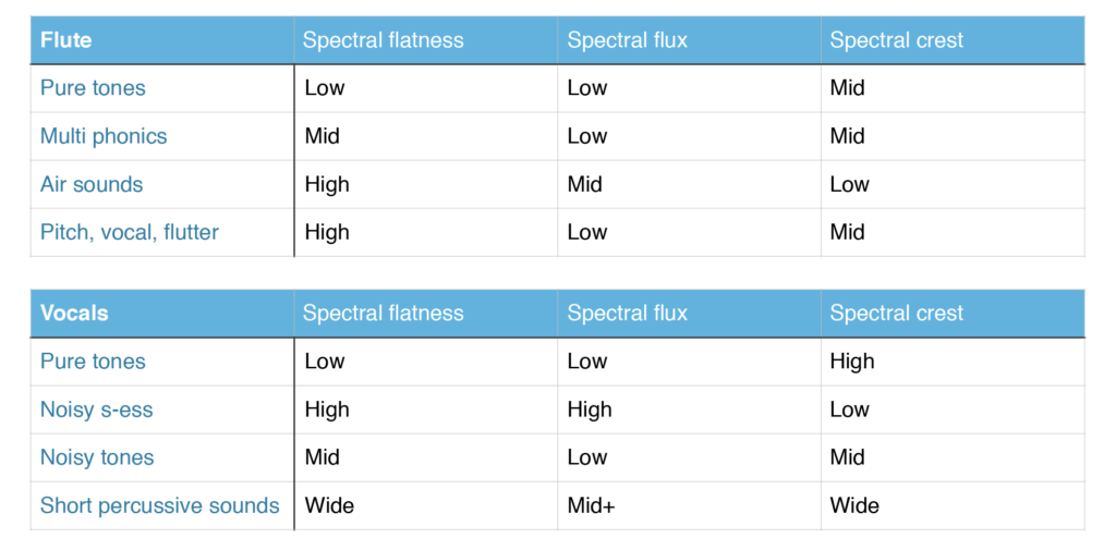
Instead of chosing analysis parameter up front, we analysed different playing techniques, e.g. non- tonal sounds (sss, shhh), multiphonics etc., and saw how the analyser responded. We also recorded short samples of the different techniques that each of us usually play, so that we could investigate the analysis several times.
This is the analysis results we got:
Since we’re all musicians experienced with live processing, we made a setup based on effects that we already know well and use in our live-electronic setup (reverb, filter, compression, ring modulation and distortion).
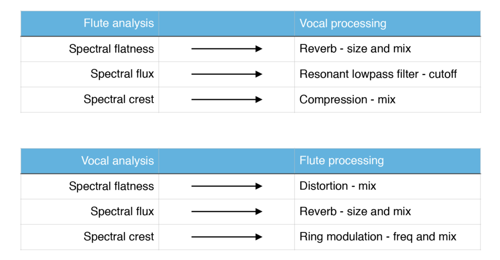
To set up meaningful mappings, we chose an approach that we entitled “spectral ducking”, where a certain musical feature on one instrument would reduce the same musical feature on the other – e.g. a sustained tonal sound produced by the vocalist, would reduce harmonic musical features of the flute by applying ring modulation. Here is a complete list of the mappings used:
Excerpt #1 – Vocal and flute
Excerpt #2 – Vocal and flute
Excerpt #3 – Vocal and flute
Excerpt #4 – Vocal and flute
Lack of consisive and presise analysis results from the guitar in combination with time limitation, it wasn’t possible to set up mappings for the guitar and flute. We did however test out the guitar and flute in the last minutes of the session, where the guitar simply took the role of the vocal in terms of processing and mapping. A knowledge of the vocal analysis and mapping, made it possible to perform with the same setup even though the input instrument had changed. Some short excerpts from this performance can be heard below.
Excerpt #5 – Guitar and flute
Excerpt #6 – Guitar and flute
Excerpt #7 – Guitar and flute
Reflections and comments:
We experienced the importance of exploring new tools like this on a known system. Since none of us knew Reaper from before, we used spent quite a lot of time learning a new system (both while preparing and during the session)
Could the meters analyser be turned the other way around? It is a bit difficult to read sideways.
It would be nice to be able to record and export control data from the analyser tool that will make it possible to use it later in a synthesis.
Could it be an idea to have more analyzer sources pr channel? The Keith McMillian Softstep mapping software could possibly be something to look at for inspiration?
The output is surprisingly musical – maybe this is a result of all the discussions and reflections we did before we did the setup and before we played?
The outcome is something else than playing with live electronics- it is immediate and you can actually focus on the listening – very liberating from a live electronics point of view!
The system is merging the different sounds in a very elegant way.
Knowing that you have an influence on your fellow musicians output forces you to think in new ways when working with live electronics.
The experience for us is that this is similar to work acoustically.
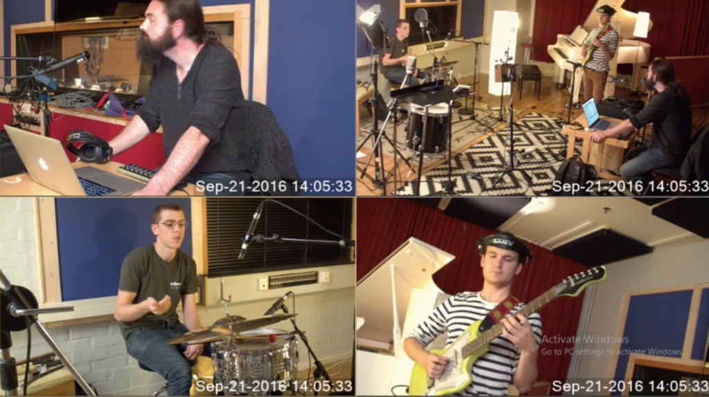
Audio and video documentaion is often an important component of projects that analyse or evaluate musical performance and/or interaction. This is also the case in the Cross Adaptive project where every session was to be recorded in video and multi-track audio, and subsequently within two days, this material should be organized and edited into a 2-5 minute digest. However, when documenting sessions in this project we face the challenge of having several musicians located in one room (the studio recording room), often so that they are facing each other rather than being oriented in the same direction. Thus, an ordinary single camera recording of the musicians would have difficulties including all musicians in one image. Our challenge, then, has been to find some way of doing this that has high enough quality to be able to detect salient aspects of the musical performances, that is in sync both for video streams and audio, and but isn’t too expensive, since the budget for this work has been limited, or too complicated to handle. In this blog post I will present some of the options I have considered, both in terms of hardware and software, and present some of the tests I have done in the process.
Commercial hardware/software solutions
One of the things we considered in the first investigative phase was to check the commercial market for multi-camera recording solutions. After some initial searches on the web I made a few inquiries, which resulted in two quotes for two different systems:
Both included all hardware and software needed for in-sync multi-camera recording, except for the cameras in themselves. The StreamPix quote also included a computer with suitable specs. Both quotes were immediately deemed inadequate since prices were well beyond our budget (> $5000).
I also have to mention that after having set up a system for the first session in September 2016, we have seen the Apollo multicamera recorder/switcher, which looks like a very light weight and convenient way of doing multi-camera recording:
At $2.995 (price listed on the US web site), it might be a possibility to consider in the future, even if it still is in the high end of our budget range.
Using PCs and USB3 cameras
A project currently running at the NTNU (in collaboration with NRK and UNINETT) is Nettmusikk (Net Music). This project is testing solutions to do high-resolution, low latency streaming of audio and video over the internet. The project has bought four USB3 cameras (Point Grey Grasshopper, GS3-U3-41C6C-C) and four dual boot (Linux/win) PCs with high-performance specs. These cameras deliver a very high quality image with low latency. However, one challenge is that the USB3 standard is still not very developed so that cameras can “plug-and-play” on all platforms, and specifically that the software and drivers for the Point Grey cameras is proprietary, and won’t therefore provide images for all software out-of-the-box.
After doing some research on the Point Grey camera solution, we found that there were several issues that made this option unsuitable and/or impractical.
1. To get full sync between cameras, they needed to have an optical strobe sync, which required a master/slave configuration with all cameras to in the same room.
2. There was no software that could do multi-camera recording from USB3 out-of-the-box. Rather, Point Grey provided an SDK (Fly Capture) with working examples that allowed building of our own applications. While this was an option we considered, it still looked like an option that demanded a bit of programming work (C++).
3. Because the cameras stream and record in raw we would also need very fast SSDs to record 4 video files at once. If we were recording 4 video streams at 8-bit 1920×1080 @ 30 FPS that would be 248.8 mb/s (62.2 x 4) of data. This would also fill up hard drive space pretty fast.
USB2 HD cameras
It turned out that one of the collaborators in the Nettmusikk project had access to four USB2 HD cameras. Since the USB2 protocol is a cross-platform standard that provides plug-and-play and usually has few issues with compatibility. The quality of these Tanberg Precision HD cameras was far from professional production quality, but had reasonably clear images. When viewing the camera image on a computer, there was a barely noticable latency. Here is a review made by the gadgeteer:
Without high-quality lenses, however, the possibilities for adjusting zoom, angle and light sensiticity were non-existent, and particularly the latter proved to be an issue in the sessions. Especially we went into problems if direct light sources were in the image, so that careful placement of light sources was necessary. Also, it was sometimes difficult to get enough distance between the cameras and the performer since the room wasn’t very big, and an adjustable lens would probably have been of help here. Furthermore, the cameras has an autofocus function that sometimes was confused in the first session, making the image blurry for a second or two, until it was appropriately adjusted. Lastly, the cameras had a foot suitable for table placement, but no possibilities of fastening it to a standard stand, like the Point Grey camera has. I therefore had to use duck tape to fasten the cameras, which worked ok, but looked far from professional.
A second issue for concern was whether these cameras could provide images with long cable lengths. What I learned here was that they would operate perfectly with an 5m USB extension if they were connected to a powered hub at the end, that provided the cameras with sufficient power. It turned out that two cameras per hub did work, but might sometimes introduce some latency and drop-outs. Thus, taking the signal from four cameras via four hubs and extension chords into the four USB ports on the PC seemed like the best solution. (Although we only used three hubs in the first session). That gave us a fairly high flexibility in terms of placing the cameras.
Mosaic image
Due to the very high amounts of data involved in dealing with multiple cameras, using instead a composite/ mosaic gathering all four images into one, seemed like a possible solution. Arguably, it would going from HD to HD/4 per image. Still, this option had the great advantage of making post-production switching between cameras superfluous. And since the goal in this project was to produce a 2-5 minute digest in two days this seemed like a very attracive option. The question was then how to collate and sync four images into one without any glitches or hiccups. In the following, I will present the four solutions that was tested:
1. ffmpeg (
https://www.ffmpeg.org/
)
ffmpeg is an open source command line software that can do a number of different operation on audio and video streams and files; recording, converting, filtering, ressampling, muxing, demuxing, etc. It is highly flexible and customizable with the cost of having a steep user threshold with cumbersome operation, since everything has to be run at command line. The flexibility and the fact that it was free still made it an option to consider.
ffmpeg could be easily installed OSX from pre built binaries. On Windows it also has to be built from sources with the mingw-w64 project (see
https://trac.ffmpeg.org/wiki/CompilationGuide/MinGW
). This option seemed like a bit of work, but at the time when it was considered, it still sounded like a viable option.
After some initial tests based on examples in the ffmpeg wiki (
https://trac.ffmpeg.org/wiki
) I was able to run the following script as a test on OSX:
The script produced four streams of video, one from the an external web camera and three from the internal Face Time HD camera. However, the individual images were far from in sync, and seemed to loose the stream and/or lag behind several seconds at a time. This initial test plus the sync issues and the prospects of a time consuming build process on Windows made me abandon the ffmpeg solution.
2. Processing
Using Processing, described as a “flexible software sketchbook and a language for learning how to code within the context of the visual arts” (
https://processing.org/
), seemed like a more promising path. Again I relied on examples I located on the web and put together a sketch that seemed to do what we were after (I also had to install the video library to be able to run the sketch).
void setup(){
size(1280, 720);
cameras=Capture.list();
println(“Available cameras:”);
for (int i = 0; i < cameras.length; i++) {
println(cameras[i], i);
}
/// Choose cameras with the appropriate number from the list and corresponding resolution
/// Here I had to look in the printout list to find the correct numbers to enter
camA = new Capture(this,640,360,cameras[18]);
camB = new Capture(this,640,360,cameras[3]);
camC = new Capture(this,640,360,cameras[33]);
camA.start();
camB.start();
camC.start();
}
void draw() {
image(camA, 0, 0, 640,360);
image(camB, 640, 0, 640,360);
image(camC, 0, 360, 640,360);
}
This sketch nicely gathered the images from three cameras into my mac, with little latency (approx. 50-100 ms). This made me opt to go further and port the sketch to Windows. After installing Processing on the win-PC and running the sktetch there however, I could only get one image out at a time. My hypothesis was that the problem came from all the different cameras having the same number in the list of drivers. These problem made me abandon Processing in search for simpler solutions.
3. IP Camera Viewer
After doing some more searches, I came across IP Camera viewer (
http://www.deskshare.com/ip-camera-viewer.aspx
), a free and light-weight application for different win versions, with support for over 2000 cameras according to their web site. After some initial tests, I found that this application was a quick and easy solution to what we wanted in the project. I could easily gather up to four camera streams in the viewer and the quality seemed good enough to capture details of the performers. It was also very easy to set up and use, and also seemed stable and robust. Thus, this solution turned out to be what we used in our first session, and it gave us results that were good enough in quality for performance analysis.
4. VLC (
http://www.videolan.org/vlc/
)
The leader of the Nettmusikk project, Otto Wittner, made a VLC script to produce a mosaic image, albeit with only two images:
# Webcam no 1
new ch1 broadcast enabled
setup ch1 input v4l2:///dev/video0:chroma=MJPG:width=320:height=240:fps=30
setup ch1 output #mosaic-bridge{id=1}
# Webcam no 2
new ch2 broadcast enabled
setup ch2 input v4l2:///dev/video1:chroma=MJPG:width=320:height=240:fps=30
setup ch2 output #mosaic-bridge{id=2}
# Background surface (image)
new bg broadcast enabled
setup bg input bg.png
# Add mosaic on top of image, encode everything, display the result as well as stream udp
setup bg output #transcode{sfilter=mosaic{width=640,height=480,cols=2,rows=1,position=1,order=”1,2″,keep-picture=enabled,align=1},vcodec=mp4v,vb=5000,fps=30}:duplicate{dst=display,dst=udp{dst=streamer.uninett.no:9400}}
setup bg option image-duration=-1 # Make background image be streamed forever
#Start everything
control bg play
control ch1 play
control ch2 play
While it seemed to work well on Linux with two images, the fact that we already had a solution in place made it natural not to persue this solution further at the time.
5. Other software
Among other software I located that could gather several images into one was CaptureSync (
http://bensoftware.com/capturesync/
). This software was for mac only, and was therefore not tested.
Screen capture and broadcast
Another important function that still wasn’t covered with the IP camera viewer was recording. Another search uncovered many options here, most of them directed towards gaming capture. The first of these I tested was OBS, Open Broadcaster Software (
https://obsproject.com/
). This open source software turned out to do exactly what we wanted and more, so this became the solution we used at the first session. The software was easily setup to record from the desktop with a 30fps frame rate and close to HD quality with output set to .mp4. There was, however, a noticable lag between audio and video, with video lagging behind approximately 50-100ms. This was corrected in post-production editing, but could potentially have been solved with inserting a delay on the audio stream until it was in sync. Also there were occasional clicks in the audio stream, but I did not have time to figure out whether this was caused by the software or the (internal) sound device we used for recording. We will do more tests on this matter later. The recordings were started with a clap to allow for post-sync.
Surprisingly, OBS was very easy to set it up for live-streaming. I used my own YouTube account where I set up for the Stream Now option (
https://support.google.com/youtube/answer/2853700?hl=en
). This gave me a a key code that I could copy into OBS, and then simply press the “Start streaming” button. The stream had a lag of about 10 seconds, but had a good quality and consistence. Thereby we had easily set up something we only considered as optional to begin with. Øyvind was very pleased to be able to follow the last part of the first session from his breakfast table in San Diego!
Live stream from session with jazz students
Custom video markup solution
Øyvind wrote a small command line program in python that could generate a time-code based list of markers to go with the video. When pressing a number one could indicate when (number of seconds before pressing) a comment was to be inserted relative to a custom set timer. This made it possible to easily synchronize with the clock that IP Camera Viewer printed on top of the video images. Moreover, it allowed rating significance. Although it required a little bit of practice, I found it useful for making notes during the session, as well as when going through the post-session interview videos. One possible way of improving it would be to have a program that could merge and order (in time) comments made either in different run throughs or by different commentators.
Editing
After two days of recording the videos were to be edited down to a single five minute video. After some testing with free software like iMovie (mac) and MovieMaker (win), I abandoned both options due to lack of options and intuitive use. After a little bit of serching I discovered Filmora from Wondershare (
http://filmora.wondershare.com/
), which I tried out as a free demo before I decided to buy it ($29.90 for a 1-year license). In my view, it was lightweight, had sufficient options to do simple editing and it was quick and easy to use.
Conclusions
We ended up with a multicamera recording and live-streaming solution that was easy to use and very cheap to set up. The only expenses we have had so far has been USB extension cords and hubs as well as the Filmora editor, which was also cheap. Although we do not have our own cameras yet, the prices of new USB2 cameras would not imply a big cut into the budget, if we need to buy four of them. Moreover, finding free software that gave us what we wanted out-of-the-box was a huge relief after intital tests with software like ffmpeg, Processing and VLC.
Participants:
Maja S. K. Ratkje, Siv Øyunn Kjenstad, Øyvind Brandtsegg, Trond Engum, Andreas Bergsland, Solveig Bøe, Sigurd Saue, Thomas Henriksen
Session objective and focus
Although the trio BRAG RUG has experimented with crossadaptive techniques in rehearsals and concerts during the last year, this was the first dedicated research session on the issues specific to these techniques. The musicians were familiar with the interaction model of live processing, the electronic modifications of the instrumental sound in real time is familiar ground. Notably, the basic concepts of feature extraction and the use of these features as modulators for the effects processing was also familiar ground for the musicians before the session. Still, we opted to start with very basic configurations of features and modulators as a means of warming up. The warm-up can be valid both for the performative attention, the listening mode, and also a way of verifying that the technical setup works as expected.
The session objective and focus is simply put to explore further the crossadaptive interactions in practice. As of now, the technical solutions work well enough to start making music, and the issues that arise during musical practice are many-faceted and we have opted not to put any specific limitations or preconceived directinos on how these explorations should be made.
As preparation for the session we (Oeyvind) had prepared a set of possible configurations (sets of features, mapped to sets of effects controllers). As the musicians was familiar with the concepts and techniques, we expected that a larger set of possible situations to be explored would be necessary. As it turned out, we spent more time investigating the simpler situations, so we did not get to test all of the prepared interaction situations. The extra time spent on the simpler situations was not due to any unforeseen problems, rather that there were interesting issues to explore even in the simpler situations, and that it seemed highly valid to explore those more fully rather than thinly testing a large set of situations. With this in mind, we could easily have continued our explorations for several more days.
The musician’s previous experience with said techniques provided an effective base for communication around the ideas, issues and problems. The musicians’ ideas were clearly expressed, and easily translated into modifications in the mapping. With regards to the current status of the technical tools, we were quickly able to do modifications to the mappings based on ad hoc suggestions during the sessions. For example changing the types of features (by having a plethora of usable features readily extracted), inverting, scaling, combining different features, gating etc. We did not get around to testing the new modulator mapping of “absolute difference” at all, so we note that as a future experiment. One thing Oeyvind notes as still being difficult is changing the modulation destination. This is presently done by changing midi channels and controller numbers, with no reference to what these controller numbers are mapped to. This also partly relates to the Reaper DAW lacking a single place to look up active modulators. It seems there are no known technologies for our MIDIator to poll the DAW for the names of the modulator destinations (the effect parameter ultimately being controlled). Our MIDIator has a “notes” field that allow us to write any kind of notesassumed to be used for jotting down destination parameter names. One obvious shortcoming of this is that it relies solely on manual (human) updates. If one changes the controller number without updating the notes, there will be a discrepancy, perhaps even more confusing than not having any notes at all.
Takes
[numbered as take 1]
Amplitude (rms_dB) on voice controls reverb time (size) on drums. Amplitude (rms_dB) on drums controls delay feedback on vocals. In both cases, higher amplitude means more (longer, bigger) effect.
Initial comments: When the effect is big on high amplitude, the action is very parallel. The energy flowing in only one direction (intensity-wise). In this particular take, the effects modulation was a bit on/off, not responding to the playing in a nuanced manner. Perhaps the threshold for the reverb was also too low, so it responded too much (even to low amplitude playing). It was a bit uncleer for the performers how much control they had over the modulations.
The use of two time based effects at the same time tends to melt things together – working against the same direction/dimension (when is this wanted unwanted in a musical situation?).
Reflection when listening to take 1 after the session: Although we now have experienced two sessions where the musicians preferred controlling the effects in an inverted manner (not like here in take 1, but like we do later in this session, f.ex. take 3), when listening to the take it feels like a natural extension to the performance sometimes to simply have more effect when the musicians “lean into it” and play loud. Perhaps we could devise a mapping strategy where the fast response of the system is to reduce the effect (e.g. the reverb time), then if the energy (f.ex. the amplitude) remains high over an extended duration (f.ex. longer than 30 seconds), then the effect will increase again. This kind of mapping strategy suggests that we could create quite intricate interaction schemes just with some simple feature extraction (like amplitude envelope), and that this could be used to create intuitive and elaborate musical forms (“form” here defined as the evolution of effects mapping automation over time.).
[numbered as take 1.2]
Same mappings as in take 1, with some fine tuning: More direct sound on drums; Less reverb on drums; Shorter release on drums’s amplitude envelope (vocal delay feedback stops sooner when drums goes from loud to soft). More nuanced disposition of vocal amplitude tracking to reverb size.
[numbered as take 1.3] Inverted mapping, using same features and same effects parameters as in take 1 and 2. Here, louder drums means less feedback of the vocal delay; Similarly, louder vocals gives shorter reverb time on the drums.
There was a consensus amongst all people involved in the session that this inverted mapping is “more interesting”. It also leads to the possibility for some nice timbral gestures; When the sound level goes from loud to quiet, the room opens up and prolongs the small quiet sounds. Even though this can hardly be described as a “natural” situation (in that it is not something we can find in nature, acoustically), it provides a musical tension of opposing forces, and also a musical potential for exploring the spatiality in relation to dynamics.
[numbered as take 2] Similar to the mapping for take 3, but with a longer release time, meaning the effect will take longer to come back after having been reduced.
The interaction between the musicians, and their intentional playing of the effects control is tangible in this take. One can also hear the drummers’ shouts of approval here and there (0:50, 1:38).
[numbered as take 3] Changing the features extracted to control the same effects . Still controlling reverb time (size) and delay feedback. Using transient density on the drums to control delay feedback for the vocals, and pitch of the vocals to control reverb size for the drums. Faster drum playing means more delay feedback on vocals. Higher vocals pitch means longer reverberation on the drums.
Maja reacted quite strongly to this mapping, because pitch is a very prominent and defining parameter of the musical statement. Linking it to control some completely other parameter brings something very unorthodox into the musical dialogue. She was very enthusiastic about this opportunity, being challenged to exploit this uncommon link. It is not natural or intuitive at all, thus being hard work for the performer, as one’s intuitive musical response and expression is contradicted directly. She would make an analogy to a “score”, like written scores for experimental music. In the project we have earlier noted that the design of interaction mappings (how features are mapped to effects) can be seen as compositions. It seems we think in the same way about this, even though the terminology is slightly different. For Maja, a composition involves form (over time), while a score to a larger extent can describe a situation. Oeyvind on the other hand uses “composition” to describe any imposed guideline put on the performer, anything that instructs the performer in any way. Regardless of the specifics of terminology, we note that the effect of the pitch-to-reverbsize mapping was effective in creating a radical or unorthodox interaction pattern.
One could crave for also testing out this kind of mapping in the inverted manner, letting transient density on the drums give less feedback, and lower pitches give larger reverbs. At this moment in the session, we decided to spend the last hour on trying something entirely different, just to have also touched upon other kinds of effects.
[numbered as take 4] Convolution and resonator effects. We tested a new implementation of the live convolver. Here, the impulse response for the convolution is live sampled, and one can start convolving before the IR recording is complete. An earlier implementation was the subject of another blog post, the current implementation being less prone to clicks during recording and considerably less CPU intensive. The amplitude of the vocals is used to control a gate (Schmitt trigger) that in turn controls the live sampling. When the vocal signal is stronger than the selected threshold, recording starts, and recording continues as long as the vocal signal is loud. The signal to be recorded is the sound of the drums. The vocal signal is used as the convolution input, so any utterance on the vocals gets convolved with the recent recording of the drums.
In this manner, the timbre of the drums is triggered (excited, energized) by the actions of the vocal. Similarly, we have a resonator capturing the timbral character of the vocal and this resonator is triggered/excited/energized by the sound of the drums. Transient density of the drums is run through a gate (Schmitt trigger), similar to the one used on the vocal amplitude. Fast playing on the drums trigger recording of the timbral resonances of the voice. The resonator sampling (one could also say resonator tuning) is a one-shot process triggered each time the drums has been playing slow and then changes to faster playing.
Summing up the mapping: Vocal amplitude triggers IR sampling (using drums as source, applying the effect to the vocals). Drums transient density triggers vocal resonance tuning (applying the effect on the drums).
The musicians liked very well playing with the resonator effect on the drums. It gave a new dimension to taking features from the other instrument and applying it to one’s own. In some way it resembles the “unmoderated” (non-cross-adaptive) improvising together, as in that setting these (these two specific) musicians also commonly borrows material from each other. The convolution process on the other hand seemed a bit more static, like one-shot playback of a sample (although it is not, it is also somewhat similar). The convolution process can also be viewed as getting delay patterns from the drum playing. Somehow, the exact patterns does not differ so much when fed a dense signal, so changes in delay patterns are not so dramatic. This can be exploited with intentionally playing in such a way as to reveal the delay patterns. Still, that is a quite specific and narrow musical situation. Other things one might expect to get from IR sampling is capturing “the full sound” of the other instrument. Perhaps the drums are not that dramatically different/dynamic to release this potential, or perhaps also the drum playing could be adapted to the IR sampling situation, putting more emphasis on different sonic textures (wooden sounds, boomy sounds, metallic sounds, click-y sounds). In any case, for our experiments in this session, we did not seem to release the full expected potential of the convolution technique.
Comments:
Most of the specific comments done for each take above, but some general remarks for the session:
Status of tools:
We seem to have more options (in the tools and toys) than we have time to explore, which is a good indication that we can perhaps relax the technical development and focus more on practical exploration for a while. It also indicates that we could (perhaps should) book practical sessions over several consecutive days, to allow more in-depth exploration.
Making music:
It also seems that we are well on the way to actually making music with these techniques, even though there is still quite a bit of resistance in the techniques. What is good is that we have found
some
situations that work well musically (for example when amplitude inversely affecting room size). Then we can expand and contrast these with new interaction situations where we experience more resistance (for example like we see when using pitch as a controller). We also see that even the successful situations appears static after some time, so the urge to manually control and shape the result (like in live processing) is clearly apparent. We can easily see that this is what we will probably do when playing with these techniques outside the research situation.
Source separation:
During this studio situation, we put the vocals and drums in separate rooms to avoid audio bleed between the instruments. This made for a clean and controlled input signal to the feature extractor, and we were able to better determine the qualitu of the feature extraction. Earlier sessions done with both instruments in the same room gave much more crosstalk/bleed and we would sometimes be unsure if the feature extractor worked correctly. As of now it seems to work reasonably well. Two days after this session, we also demonstrated the techniques on stage with amplification via P.A. This proved (as expected) very difficult due to a high degree of bleed between the different signals. We should consider making a crosstalk-reduction processor. This might be implemented as a simple subtraction of one time-delayed spectrum from the other, introducing additional latency to the audio analysis. Still, the effects processing for audio output need not be affected by the additional latency, only the analysis. Since many of the things we want to control change relatively slowly, the additional latency might be bearable.
Trond Engum, Andreas Bergsland, Tone Åse, Thomas Henriksen, Oddbjørn Sponås, Hogne Kleiberg, Martin Miguel Almagro, Oddbjørn Sponås, Simen Bjørkhaug, Ola Djupvik, Sondre Ferstad, Björn Petersson, Emilie Wilhelmine Smestad, David Anderson, Ragnhild Fangel
Session objective and focus:
This post is a description of a session with 3rd year Jazz students at NTNU. It was the first session following the intended procedure framework for documentation of sound and video in the cross adaptive processing project. The session was organized as part of the ensemble teaching that is given to Jazz students at NTNU, and was meant to take care of both the learning outcomes from the normal ensemble teaching, and also aspects related to the cross adaptive project. This first approach was meant as a pilot for the processing musician and the video and documentation aspect. It can also be seen as a test on how musicians not directly involved in the project react and reflect within the context
of cross adaptive processing.
We made a choice to keep the processing system as simple as possible to make the technical aspect of the session as understandable as possible for all parts involved. To achieve this we only used analyses of RMS and transient density on the instruments to link conventional instrumental performance close to how the effects were controlled. As an example: The louder you play either the more or less of one effect is heard, or depending on the transient density the more or less of one effect is heard. All instruments were set up to control the amount of processed signal on two different effects each, giving the system a potential to use up to four different effects at the same time. The processing musician had a possibility to adjust the balance between the different processed signals during performance. The direct signal from the instruments was also kept as part of the mix to reduce an alienation from the acoustic sound of the instrument since this was a first attempt for those involved. Since the musicians, besides performing on their instruments, also indirectly perform the sound production we chose to follow up a premise of a shared listening strategy used by the T-Emp ensemble.
https://www.researchcatalogue.net/view/48123/53026
The basic idea is that if everyone hears the same mix, they will adjust individually and consequently globally to the sound image as a whole through their instrumental and sound production output.
Sound examples:
Besides normalising, all sound examples presented in this post are unprocessed and unedited in postproduction meaning that they have the same mix between instruments and processing as the musicians and observers auditioned during recording.
20.09.2016
Take 1 – Session 20.09.16 take 1 drums_piano.wav
Drums and piano
Drums controlling the volume of how much overdrive or reverb is added to the piano. The analysing parameters used on the drums are rms_dB and trans_dens. The louder the drums play, the more overdrive on the piano, and the larger transient density the less reverb on the piano. The take has some issues with bleeding between microphones since both performers are in the same room.
There was also a need for fine-tuning the behaviour of both effects through the rise and fall parameters in the mediator plug in during the take.
Even though it would be natural to presume that more is more in a musical interplay – for example that the louder you play the more effect you receive – the performers experienced that more is less was more convenient on the reverb in this particular setting. It felt natural for the musicians that when the drummer played faster (higher degree of transient density) the amount of reverb on the piano was decreased. After this take we had a system crash. As a consequence the whole set up was lost, and a new set up was built from scratch for the rest of the session.
Take 2
– Session 20.09.16 take 2
drums_piano.wav
Drums and piano
The piano controlling the loudness on the amount of echo and reverb are added to the drums. The larger transient density the more echo on drums, the louder piano the more reverb on the drums.
Take
3
– Session 20.09.16 take
3
drums_piano.wav
The piano controlling the volume of how much echo and reverb are added to the drums. The larger transient density the more echo on drums, the louder piano the more reverb on the drums. Loudness on drums controls overdrive on piano (the louder the more overdrive), and transient density controls reverb – the larger transient density the less reverb on the piano.
21.09.2016
Due to technical challenges the first day we made some adjustments on the system in order to avoid the most obvious obstacles. We changed from condenser to dynamic microphones to decrease the amount of bleeding between them (bleeding affects the analyser plug-in and also adds the same effect to both instruments, as experienced earlier in the project). The reason for the system crash was identified in the Reaper setup, and a new template was also made in Ableton live. We chose to keep the set up simple during the session to clarify the musical results (Only two analysing parameters controlling two different effects on each instrument).
Take 1 – Session 21.09.16 take 1 drums_guitar.wav
Percussion and guitar
Percussion controlled the amount of effect on the guitar using rms-dB and trans-dens as analysis parameters – the louder percussion, the more reverb on the guitar, and the larger the transient density on percussion, the more echo on the guitar. This set up was experienced as uncomfortable for the performers, especially when loud playing resulted in more reverb. There was still an issue with bleeding even though we had changed to dynamical microphones.
Take 2 – Session 21.09.16 take 2 drums_guitar.wav
We agreed upon some changes suggested by the musicians. We used the same analysis parameters on the percussion, with percussion controlling the amount of effect on the guitar, using rms-dB and trans-dens: The louder percussion, the less overdrive on guitar, and the larger transient density of the percussion, the more echo on guitar. This resulted in a more comfortable relationship between the instruments and effects seen from the performers perspective.
Take 3 – Session 21.09.16 take 3 drums_guitar.wav
This setup was constructed to interact both ways through the effects applied to the instruments. We used the same analysis parameters on the percussion with percussion controlling the amount of effect on the guitar, using rms-dB and trans-dens: The louder percussion, the less overdrive on guitar, and the more transient density of the percussion, the more echo on guitar. We used the same analysis parameters on the guitar as on the percussion (rms-dB and trans-dens): The louder guitar, the more overdrive on percussion, and larger transient density on guitar the more reverb on percussion. During this session the percussionist also experimented with the distance to the microphones to test out movement and proximity effect in connection with the effects. The trans-dens analyses on the guitar did not work as dynamically as expected due to some technical issues during the take.
Take 4 – Session 21.09.16 take 4 harmonica_bass.wav
Double bass and harmonica
We started out with letting the harmonica control the effects on the double bass based using the analyses of rms-dB and trans_dens. The more harmonica volume, the less overdrive on bass, and the more transient density on the harmonica, the more echo on bass. This first take was not very successful due to bleeding between microphones (dynamical). There was also an issue with the fine-tuning in the mediator concerning the dynamical range sent to the effects. This resulted in a experience that the effects where turned on and off, and not changed dynamically over time which was the original intention. There was also a contradiction between musical intention and effects. (The harmonica playing louder reducing overdrive on the bass)
Take 5 – Session 21.09.16 take 5 harmonica_bass.wav
Based on suggestions by the musicians we set up a system controlling effects both ways. The harmonica still controlled the effects on the double bass based on the analyses of rms-dB and trans_dens, but now we tried the following: The more harmonica volume, the more overdrive on bass, and the more transient density, the more echo on bass. The bass used analyses of two instances of rms-dB to control the effects on the harmonica: The louder the bass, the less reverb on the harmonica, and the louder the bass the more overdrive on the harmonica. This set created a much more “intuitive” musical approach seen from the performers perspective. The function with the harmonica controlling the bass overdrive worked against the performers musical intention, and this functionality was removed during the take. This should probably not have been done during a take, but it was experienced as a bit confusing for the instrumentalists in this setting. This take show how dependent the musicians are on each other in order to “activate” the effects, and also the relationship and potential between musical energy followed up by effects.
Take 6 – Session 21.09.16 take 6 vocals_saxophone.wav
Vocals and Saxophone
In this setup the saxophone controls the effects on the vocals based on two instances of rms_dB analyses: The louder the saxophone, the less reverb on the vocals, and the louder the saxophone, the more echo is added to the vocals. The first attempt had some problems with the balance between dry and wet signal in the mix from the control room. The vocal input was lower compared to sources present earlier that day. As a consequence, the saxophone player was unable to hear both the direct signal of the voice, but also the effects he added to the voice. This was tried compensated for during the take by boosting the volume of the echo during the take, but without any noticeable result in the performance. Another challenge that occurred in this take was a result of the choice of effects. Both reverb and echo can sound quit similar on long vocal notes, and as a consequence blurred the experienced amount of control over the effects. This pinpoints the importance of good listening conditions for the musicians in this project, especially if working with more subtle changes in the effects.
Take 7 – Session 21.09.16 take 7 vocals_saxophone.wav
Before recording a new take we made adjustments in the balance between wet and dry sound in the control room. We then did a second take with the same settings as take 6. It was clear that the performers took more control over the situation because of better listening conditions. The performers expressed a wish to practise with the set up on beforehand. Another aspect that was asked for by the performers was that the system should open up for subtle changes in the effects while still keeping the potential to be more radical at the same time depending on the instrumental input. The saxophone player also mentioned that it could be interesting to add harmonies as one of the effects since both instruments are monophonic.
Take 8 – Session 21.09.16 take 8 vocals_saxophone.wav
The last take of the day included the vocals to control the effects on the saxophone. The saxophone was kept with the same system as in the two former takes: The louder the saxophone, the less reverb on the vocals, and the louder the saxophone, the more echo was added to the vocals. The vocals were analysed by rms_dB and trans_dens: The more loudness on vocals, the more overdrive on saxophone, and the larger transient density on the vocals, the more echo on the saxophone. Both performers experienced that this system was meaningful both musically and in aspect of control over the effects. They communicated that there was a clear connection between the musical intention and the sounding result.
Comments:
All the involved musicians communicated that the experiment was meaningful even though it was another way of interacting in a musical interplay. The performers want to try this more with other set ups and effects. Even though this was the first attempt for the performers and the processing musician we achieved some promising musical results.
Technical issues to be solved:
There are still some technical issues to be solved in the software (first of all avoiding system crashes during sessions). Bleeding between microphones is also an issue that needs to be attended to. (This challenge will be further magnified in a live setting).
On/off control versus dynamical control, We need more time together with the performers to rehearse and fine – tune the effects.
Performers involved need more time together with the processing musician to rehearse before takes in order to familiarize with the effects and how they affect them.
The performers experience of being in control/not being in control of the effects.
Other thoughts from the performers:
Suggestions about visual feedback and possibility to make adjustments directly on the effects themselves.
It could be interesting to focus just as much on removing attributes from the effects through instrumental control as adding. (Adding more effects is often the first choice when working with live electronics.
Agree upon an aesthetical framework before setting up the system involving all performers.