Adding new array operations to Csound II: the Mel-frequency filterbank

As I have discussed before in my previous post, as part of this project we have been selecting a number of useful operations to implement in Csound, as part of its array opcode collection. We have looked at the components necessary for the implementation of the Mel-frequency cepstrum coefficient (MFCC) analysis and in this post I will discuss the Mel-frequency filterbank as the final missing piece.

The word filterbank might be a little misleading in this context, as we will not necessarily implement a complete filter. We will design a set of weighting curves that will be applied to the power spectrum. From each one of this we will obtain an average value, which will be the output of the MFB at a given centre frequency. So from this perspective, the complete filter is actually made up of the power spectrum analysis and the MFB proper.

So what we need to do is the following:

  1. Find L evenly-space centre frequencies in the Mel scale (within a minimum and maximum range).
  2. Construct L overlapping triangle-shape curves, centred at each Mel-scale frequency.
  3. Apply each one of these curves to the power spectrum and averaging the result. These will be the outputs of the filterbank.

The power spectrum input comes as sequence of equally-spaced bins. So, to achieve the first step, we need to convert to/from the Mel scale, and also to be able to establish which bins will be equivalent to the centre frequencies of each triangular curve. We will show how this is done using the Python language as an example.

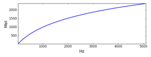
The following function converts from a frequency in Hz to a Mel-scale frequency.

import pylab as pl
def f2mel(f):
  return 1125.*pl.log(1.+f/700.)

mel

With this function, we can convert our start and end Mel values and linearly space the L filter centre frequencies. From these L Mel values, we can get the power spectrum bins using

def mel2bin(m,N,sr):
  f = 700.*(pl.exp(m/1125.) - 1.)
  return  int(f/(sr/(2*N)))

where m is the Mel frequency, N is the DFT size used and sr is the sampling rate. A list of bin numbers can be created, associating each L Mel centre frequency with a bin number

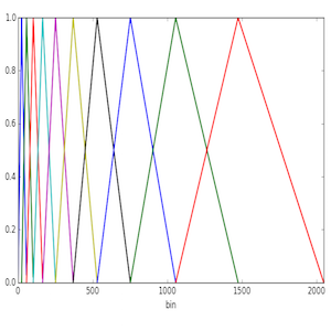
Step 2 is effectively based on creating ramps that will connect each bin in the list above. The following figure demonstrates the idea for L=10, and N=4096 (2048 bins)

mfb
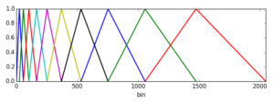
Each triangle starts at a Mel frequency in the list, rises to the next, and decays to the following one (frequencies are quantised to bin centres). To obtain the output for each filter we weigh the bin values (spectral powers) by these curves and then output the average value for each band.

The Python code for the MFB operation is shown below:

def MFB(input,L,min,max,sr):
  """
  From a power spectrum in input, creates an array 
  consisting of L values containing
  its MFB, from a min to a max frequency sampled 
  at sr Hz.
  """
  N = len(input)
  start = f2mel(min)
  end = f2mel(max)
  incr = (end-start)/(L+1)
  bins = pl.zeros(L+2)
  for i in range(0,L+2):
    bins[i] = mel2bin(start,N-1,sr)
    start += incr
  output = pl.zeros(L)
  i = 0
  for i in range(0,L):
    sum = 0.0
    start = bins[i]
    mid = bins[i+1]
    end = bins[i+2]
    incr =  1.0/(mid - start)
    decr =  1.0/(end - mid)
    g = 0.0
    for bin in input[start:mid]:
      sum += bin*g
      g += incr
    g = 1.0
    for bin in input[mid:end]:
      sum += bin*g
      g -= decr
    output[i] = sum/(end - start) 
  return output

We can demonstrate the use of the MFB  by plotting the output of a N=4096, L=128 full-spectrum magnitude analysis of a flute tone.
mfb2

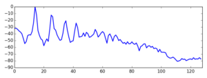
We can see how the MFB identifies clearly the signal harmonics. Of course, the original application we had in mind (MFCCs) is significantly different from this one, but this example shows what kinds of outputs we should expect from the MFB.

Adding new array operations to Csound I: the DCT

As we started the project, Oeyvind and myself were discussing a few things we thought should be added directly to Csound in order to allow more efficient signal analysis. The first of these things we looked at were components to allow Mel Frequency Cepstral Coefficients (MFCCs) to be calculated.

We have already various operations on arrays, to which I thought could we could add other things, so that we have all the components necessary for MFCC computation. The operations we need for MFCCs are:

– windowed Discrete Fourier Transform (DFT)
– power spectrum
– Mel-frequency filterbank
– log
– Discrete Cosine Transform (DCT)

Window -> DFT -> power spectrum -> MFB -> log -> DCT -> MFCCs

Of these, we had everything in place but the filterbank and the DCT. So I went off to add these two operations. I’ll spend some time in this post discussing some features of the DCT and the process of implementing it.

The DCT is one of these operations a lot of people use but do not understand it well. The earliest mention I see of it in the literature is on a paper by Ahmed, Natarajan and Rao, “Discrete Cosine Transform” , where one of its forms (the type-II DCT) and its inverse are presented. Of course, the idea originates from the so-called half-transforms, which include the continuous-time, continuous-frequency Cosine Transform and the Sine Transform, but here we have a fully discrete-time discrete-frequency operation.

In general, we would expect that a transform whose bases are made up of cosines would correctly pick up on cosine-phase components of a signal and so does the DCT. However, this is only part of the history, because implied in this is that a signal will be modelled by cosines, so that what we are trying to do is to think of this as a periodically repeated function with even boundaries (“symmetric” or “mirror-like”). In other words, that its continuation beyond the particular analysis window is modelled as even. The DFT, for instance, does not assume this particular condition, but only models the signal as a single cycle of a waveform (with the assumption that it is repeated periodically).

This assumption of evenness is very important. It means that we expect something of the waveform in order to model it cleanly, but that might not always be possible. Let’s think of two cases: cosine and sine waves. If we take a DFT and its magnitude spectrum of one full cycle of these functions, we will detect a component in bin 1 in both cases, as expected

cos-sin-dft

With DCT, however, because it assumes even boundaries, we only get a clean analysis of the cosine wave (because it is even), whereas the sine (which is odd) gets smeared all over the lower-order bins:

cos-sin-dct

Note also that in the cosine case, the component is picked up by bin 2 (instead of bin 1). This can be explained by the fact that the series used by the DCT is based on multiples of a 1/2-cycle cosine (see the expression for the transform below) and so a full-period wave is actually detected in the second analysis frequency point.

So the analysis is not particularly great in the case of non-symmetric inputs, but it actually does what it says on the tin: it models the signal as if it were made of a sum of cosines. The data can also be inverted back to the time domain, so we can recover the original signal. Despite these conditions, the DCT is used in many applications where its characteristics are appropriately useful. One of these is in the computation of the MFCCs as outlined above, because in this process we are using the power spectrum (split into a smaller number of bands by the MFB) as the input to the DCT. Since audio signals are real-valued, this is an even function and so we can model it very well with this transform.

In the case of the DCT II, which we will be implementing, the signal is assumed to be even at both the start and end boundaries. In addition, the point of symmetry is placed halfway between the first signal sample and its implied predecessor, and halfway between the last sample and its implied successor. This also implies a half-sample delay in the input signal, something that is clearly seen in the expression for the transform:

dct

Finally, when we come to implement it, there are two options. If we have a DCT available in one of the libraries we are using, we can just employ it directly. In the case of Csound, this is only available in one of the platforms (OSX through the accelerate framework) and so we have to use our second option: re-arrange the input data and apply it to a real-signal DFT.

The DCT II is equivalent (disregarding scaling) to a DFT of 4N real inputs, where we re-order the input data as follows:

dct-dft

where y(n) is the input to the DFT and x(n) is the input to the DCT. You can see that all even-index samples are 0 and the input data is placed in the odd samples, symmetrically about the centre of the frame. For instance if the DCT input is  [1,2,3,4], the DFT input will be [0,1,0,2,0,3,0,4,0,4,0,3,0,2,0,1]. Once this re-arrangement is done, we can take the DFT and then scale it by 1/2.

For this purpose, I added a couple of new functions to the Csound code base, to perform the DCT as outlined above and its inverse operation. These use the new facility where the user can select the underlying FFT implementation, either the original fftlib, PFFFT, or accellerate (veclib, OSX and iOS only) via an engine option. To make this available in the Csound language, two new array operations were added:

i/kOut[] dct  i/kSig[]   and   i/kOut idct i/kSpec[]

With these, we are able to code the final step in the MFCC process. In my next blogpost, I will discuss the implementation of the Mel-frequency filterbank, which completes the set of operators needed for this algorithm.

Evolving Neural Networks for Cross-adaptive Audio Effects

I’m Iver Jordal and this is my first blog post here. I have studied music technology for approximately two years and computer science for almost five years. During the last 6 months I’ve been working on a specialization project which combines cross-adaptive audio effects and artificial intelligence methods. Øyvind Brandtsegg and Gunnar Tufte were my supervisors.

A significant part of the project has been about developing software that automatically finds interesting mappings (neural networks) from audio features to effect parameters. One thing that the software is capable of is making one sound similar to another sound by means of cross-adaptive audio effects. For example, it can process white noise so it sounds like a drum loop.

Drum loop (target sound):

White noise (input sound to be processed):

Since the software uses algorithms that are based on random processes to achieve its goal, the output varies from run to run. Here are three different output sounds:

These three sounds are basically white noise that have been processed by distortion and low-pass filter. The effect parameters were controlled dynamically in a way that made the output sound like the drum loop (target sound).

This software that I developed is open source, and can be obtained here:

https://github.com/iver56/cross-adaptive-audio

It includes an interactive tool that visualizes output data and lets you listen to the resulting sounds. It looks like this:

visualization-screenshot
For more details about the project and the inner workings of the software, check out the project report:

Evolving Artificial Neural Networks for Cross-adaptive Audio (PDF, 2.5 MB)

Abstract:

Cross-adaptive audio effects have many applications within music technology, including for automatic mixing and live music. The common methods of signal analysis capture the acoustical and mathematical features of the signal well, but struggle to capture the musical meaning. Together with the vast number of possible signal interactions, this makes manual exploration of signal mappings difficult and tedious. This project investigates Artificial Intelligence (AI) methods for finding useful signal interactions in cross-adaptive audio effects. A system for doing signal interaction experiments and evaluating their results has been implemented. Since the system produces lots of output data in various forms, a significant part of the project has been about developing an interactive visualization tool which makes it easier to evaluate results and understand what the system is doing. The overall goal of the system is to make one sound similar to another by applying audio effects. The parameters of the audio effects are controlled dynamically by the features of the other sound. The features are mapped to parameters by using evolved neural networks. NeuroEvolution of Augmenting Topologies (NEAT) is used for evolving neural networks that have the desired behavior. Several ways to measure fitness of a neural network have been developed and tested. Experiments show that a hybrid approach that combines local euclidean distance and Nondominated Sorting Genetic Algorithm II (NSGA-II) works well. In experiments with many features for neural input, Feature Selective NeuroEvolution of Augmenting Topologies (FS-NEAT) yields better results than NEAT.

Seminar and meetings at Queen Mary University of London

June 9th and 10th we visited QMUL, met Joshua Reiss and his eminent colleagues there.  We were very well taken care of and had a pleasant and interesting stay.  June 9th we had a seminar presenting the project, and discussing related issues with a group of researchers and students. The seminar was recorded on video, to be uploaded on QMUL youtube. The day after we had a meeting with Joshua, going in more detail. We also got to meet several PhD students and got insight into their research.

Seminar discussion

Here’s some issues that were touched upon in the seminar discussion:

* analyze gestures inherent in the signal, e.g. crescendo, use this as trigger, to turn some process on or off, flip a preset etc. We could also analyze for very specific patterns, like a melodic fragment, but probably better to try to find gestures that can be performed in several different ways, so that the musician can have freedom of expression while providing a very clear interface for controlling the processes.

* Analyze features related to specific instruments. Easier to find analysis methods to extract very specific features. Rather than asking for “how can we analyze this to extract something interesting… This is perhaps a lesson for us to be a bit more specific in what we want to extract. This is somewhat opposite to our current exploratory effort in just trying to learn how the currently implemented analysis signals works and what we can get from them.

* Look for deviations from a quantized value. For example pitch deviations within a semitone, and rhythmic deviations from a time grid.

* Semantic spaces. Extract semantic features from the signal, could be timbral descriptors, mood, directions etc. Which semantics? Where to take the terminology from? We should try to develop examples of useful semantics, useful things to extract.

* Semantic descriptors are not necessarily a single point in a multidimensional space, it is more like a blob, and area. Interpolation between these blobs may not be linear in all cases. We don’t have to use all implied dimensions, so we can actually just select features/semantics/descriptors that will give us the possibility of linear interpolation. At least in those situations where we need to interpolate…

* Look at old speech codexes. Open source. Exitation/resonator model, LPC.  This is time domain, so will be really fast/low-latency.

* Cepstral techniques can also be used to separate resonator and exciter. The smoothed cepstrum being the resonator. Take the smoothed cepstrum and subtract it from the full cepstrum to get the excitation.

* The difficulty of control. The challenge to the performer, limiting the musical performance,  inhibiting the natural ways of interaction. This is a recurring issue, and something we might want to take care to handle carefully. This is also really what the project is about: creating *new* ways of interaction.

* Performer will adapt to imperfections of the analysis. Normally, MIR signals are not “aware” that they are being analyzed. They are static and prerecorded. In our case, the performer, being aware of how the analysis method works and what it responds to, can adapt the playing to trigger the analysis method in highly controllable manners. This way the cross-adaptivity is not only technical related to the control of parameters, but adaptive in relation to how the performer shapes her phrases and in turn also what she selects to play.

* Measuring collective features. Features of the mix. Each instrument contributes equally to the modulator signal. One signal can push others down or single them out. Relates to game theory. What is the most favorable behavior over time: suppress others or negotiate and adapt.

Meeting with Joshua

* Josh mentioned a few researchers that we might be interested in. Brech de Man: Intelligen audio switcher. Emannuel Chourdakis: Feature based reverb.  Dave Ronan: Groups, stems, automatic mixing. Vincent Verfaille: effect classification and A-DAFX. Brian Pardo: interfaces for music performance/production, visualization, semantics, machine learning. Pedro Pestana: sound engineer, best practices (phD), automatic mixing. Ryan Stables: SAFE plugins.

* Issues relating to publishing our work and getting an audience for it. As we could in some respect claim to create a new field, creating a community for it might be essential for further use of our research. Increase visibility. Promote also via QMUL press and NTNU info. Among connected fields are Human Computer Interaction, New Instruments for Musical Expression, Audio Engineering Society.

* QMUL has considerable experience in evaluation studies, user experience tests, listening tests etc. Some of this may be beneficial as a perspective on our otherwise experiental approach.

* Collective features (meaning individual signals in relation to each other and to the ensemble mix): Masking (spectral overlap). Onset times in relation to other instruments, lagging. Note durations, percussive/sustained etc.

* We currently use spectral crest, but crest also being useful in the time domain to do rhythmic analysis (rhythmic density, percussiveness, dynamic range). Will work better with loudness matching curve (dB)

* Time domain filterbank faster than FFT. Logarithmically spaced bands

* FFT of the time domain amp envelope

* Separate silence from noise. Automatic gain control. Automatic calibration of noise floor (use peak to average measure to estimate what is background noise and what is actual signal)

* Look for patterns: playing the same note, also pitch classes (octaves), also collectively (between instruments).

* Use log freq spectrum, and amps in dB, then do centroid/skew/flux etc

* How to collaborate with others under QMUL, adapting their plugins. Port the techniques to Csound or re-implement ours in C++? For the prototype and experimentation stage maybe modify their plugins to output just control signals? Describe clearly our framework so their code can be plugged in.


Seminar at De Montfort


Simon_and_Leigh
Simon and Leigh in Leigh’s office at De Montfort

Wednesday June 8th we visited Simon Emmerson at De Montfort and also met Director Leigh Landy. We were very well taken care of and had a pleasant and interesting stay. One of the main objectives was to do seminar with presentation of the project and discussion among the De Montfort researchers. We found that their musical preference seems to overlap considerably with our own, in the focus on free improvisation and electroacoustic art music. As this is the most obvious and easy context to implement experimental techniques (like the crossadaptive ones) we had taken care to also present examples of use within other genres. This could be interpreted as if we were more interested in traditional applications/genres than the free improvised genres. Now knowing the environment at Leicester better, we could probably have put more emphasis on the free electroacoustic art music applications. But indeed this led to interesting discussions about applicability, for example:

*In metric /rhythmic genres, one could easier analyze and extract musical features related to bar boundaries and rhythmic groupings.

* Interaction itself could also create meter, as the response time (both human and technical), has a rhythm and periodicity that can evolve musically due to the continuous feedback processes built into the way we interact with such a system and each other in the context of such a system..

* Static and deterministic versus random mappings. Several people was interested in more complex and more dynamic controller mappings, expressing interest and curiosity towards playing within a situation where the mapping could quickly and randomly change. References were made to Maja S.K. Ratkje and that her kind of approach would probably make her interested in situations that were more intensely dynamic.  Her ability to respond to the challenges of a quickly changing musical environment (e.g. changes in the mapping) also correlating with an interest to explore this kind of complex situations.  Knowing Maja from our collaborations, I think they may be right, take note to discuss this with her and try to make some challenging mapping situations for her to try out.

* it was discussed whether the crossadaptive methods could be applied to the “dirty electronics” ensemble/course situation, and there was an expressed interest in exploring this. Perhaps it will be crossadaptivity in other ways than what we use directly on our project, as the analysis and feature extraction methods does not necessarily transfer easily to the DIY (DIT – do it together, DIWO – Do it with others) domain. The “Do it with others” approach resonates well with what we generally approach btw.

* The complexity is high even with two performers. How many performers do we envision this to be used with? How large an ensemble? As we have noticed ourselves also, following the actions of two performers somehow creates a multi-voice polyphonic musical flow (2 sources, each source’s influence on the other source and the resulting timbral change resulting thereof, and the response of the other player to these changes). How many layers of polyphony can we effectively hear and distinguish when experiencing the music? (as performers or as audience). References were made to the laminal improvisation techniques of AMM.

* Questions of overall form. How will interactions under a crossadaptive system change the usual formal approach of a large overarching rise and decay form commonly found in “free” improvisation, At first I took the comment to suggest that we also could apply more traditional MIR techniques of analyzing longer segments of sound to extract “direction of energy” and/or other features evolving over longer time spans. This could indeed be interesting, but also poses problems of how the parametric response to long-terms changes should act (i.e. we could accidentally turn up a parameter way too high, and then it would stay high for a long time before the analysis window would enable us to bring it back down). Now, in some ways this would also resemble using extremely long attack and decay times for the low pass filter we already have in place in the MIDIator, creating very slow responses, needing continued excitation over a prolonged period before the modulator value will respond. After the session, I discussed this more with Simon, and he indicated that the large form aspects were probably just as much meant with regards to the perception of the musical form, rather than the filtering and windowing in the analysis process. There are interesting issues of drama and rhetoric posed by bringing these issues in, whether one tackles them on the perception level or the analysis and mapping stage.

* Comments were made that performing successfully on this system would require immense effort in terms of practicing and getting to know the responses and the reactions of the system in such an intimate manner that one could use it effectively for musical expression.  We agree of course.